./articles/ Understanding Spatial Indexing Trees
This post explores three fundamental structures, KDTrees, BallTrees, and the STR-packed R-tree, moving beyond scikit-learn imports to understand their mathematical backbones. We will dissect how they slice the Euclidean plane (and hyperspace), why the "Curse of Dimensionality" breaks some but not others.
Quick Navigation
1. Foundations of Spatial Partitioning
The starting point for all three structures (KDTree, BallTree, STR-packed R-tree) is the same: avoid scanning everything.
Given a set of \(N\) geometric objects (points, line segments, polygons) in a domain \(X \subset \mathbb{R}^d\), the baseline way to answer a query is to check the query against all objects. For example:
-
Range query: given a region \(R \subset
\mathbb{R}^d\), return all objects intersecting \(R\).
Example: Find all restaurants within a 1 km radius of a location. -
k-nearest neighbor (kNN): given a query point \(q \in
\mathbb{R}^d\), find the \(k\) objects with minimum distance \(d(q,
\cdot)\).
Example: Find the 5 closest ATMs to the user's current position.
A naive implementation is \(O(N)\) per query. Spatial trees are hierarchical filters that try to achieve something closer to \(O(\log N)\) query time (for fixed, low dimension and "nice" distributions) by eliminating large chunks of space or data at once.
The Core Idea: Prune by Geometry, Not by IDs
All three structures can be viewed as trees where each node represents a region of space that contains some subset of the data. Very informally:
-
KDTree: recursively cuts space with axis-aligned
hyperplanes (what does it mean? Don't worry we see that in the next
chapter).
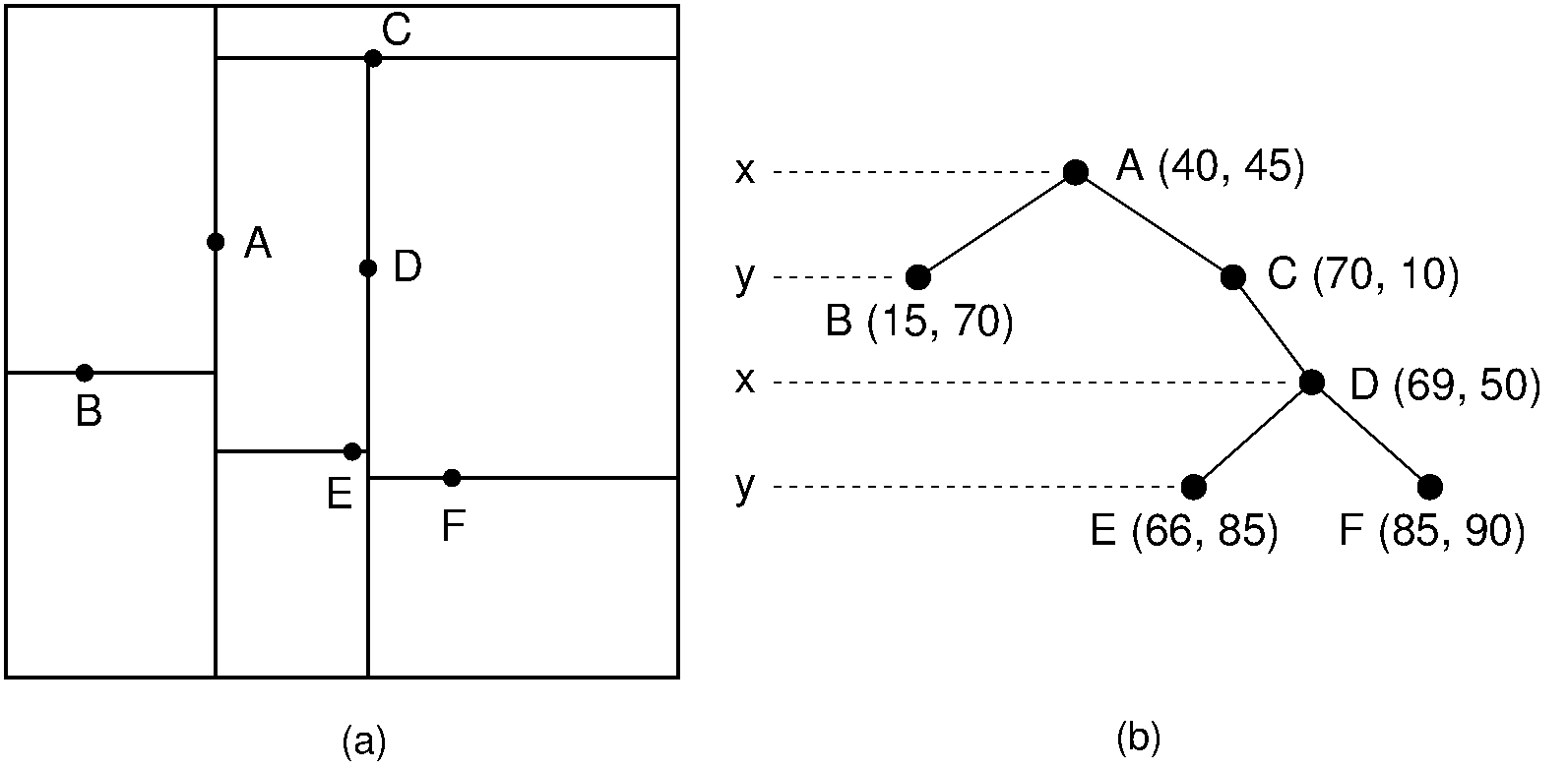
KDTree Structure -
BallTree: recursively groups points into nested
metric balls (Again, we will discuss later).
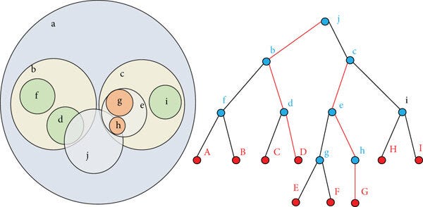
BallTree Structure -
R-tree / STRtree: recursively groups objects into
bounding rectangles (or boxes in higher \(d\)).
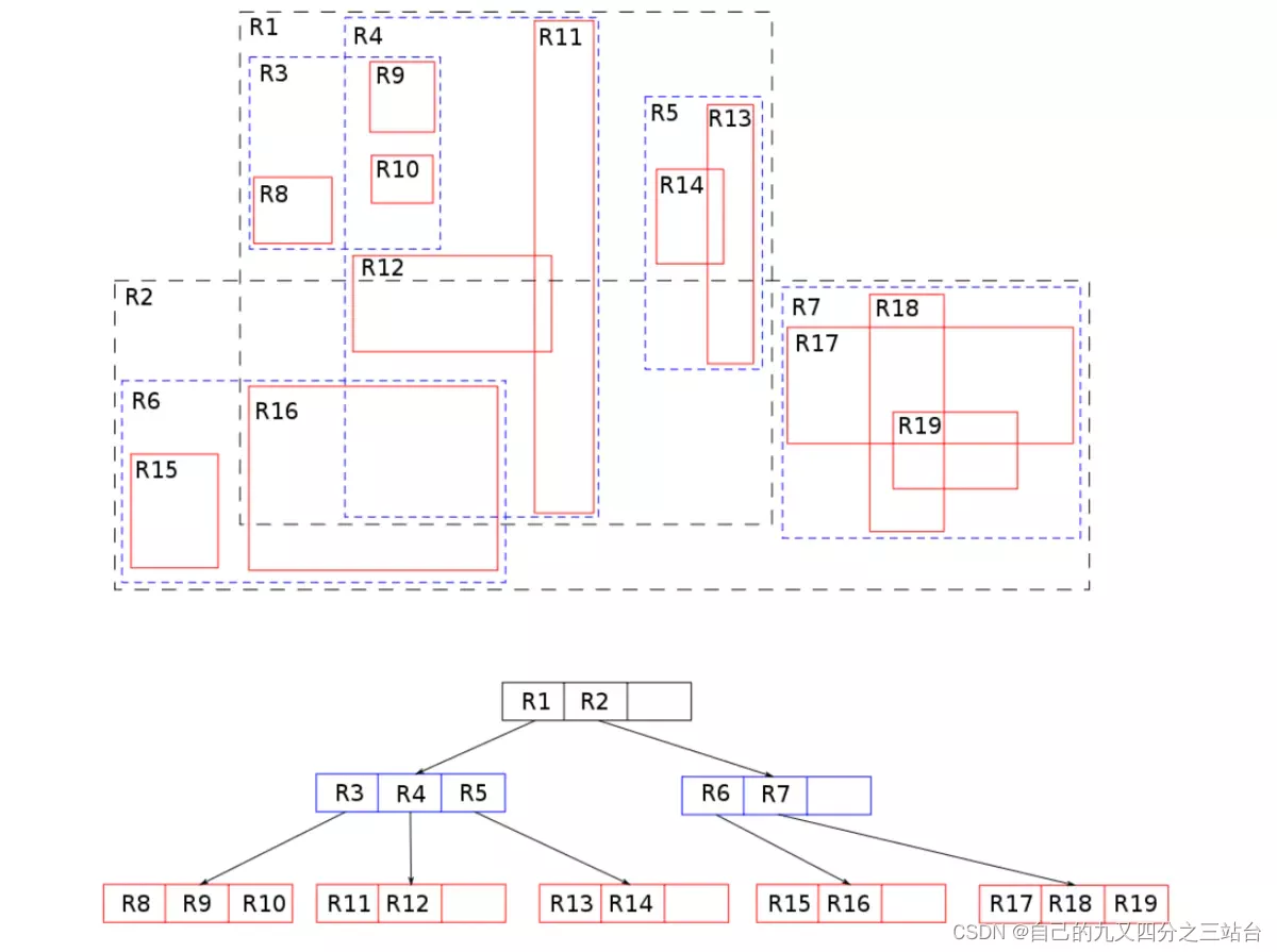
R-tree Structure
The query algorithm then walks the tree and repeatedly answers: "Can this entire region be safely ignored?" If yes, the entire subtree is pruned in \(O(1)\), rather than scanning all contained objects.
Space-Partitioning vs Data-Partitioning
A useful conceptual distinction:
Space-partitioning indexes (KDTree, quadtrees, etc.):
- Partition the geometric space \(X\) itself into disjoint regions (cells).
- Every point falls into exactly one region at each level.
- Nodes correspond to regions of \(X\), regardless of how many points are there.
Data-partitioning indexes (R-tree, BallTree and variants):
- Partition the set of objects into groups.
- For each group, store a bounding region that encloses exactly the members of that group.
- Nodes correspond to groups of objects and their bounding shapes.
This has practical consequences:
- In space-partitioning, you may get empty regions if space is sparsely populated.
- In data-partitioning, every node corresponds to at least one object, but bounding regions can overlap.
Later, this will map nicely to:
- KDTree: clean partitions of \(\mathbb{R}^d\) with hyperplanes.
- BallTree: nested metric balls around point clusters.
- STRtree: packed groups of objects in minimum bounding rectangles (MBRs).
Formal Setup: Metric Space and Queries
Assume a metric space \((X, d)\):
- \(X\) is the set of objects (often \(X = \mathbb{R}^d\)).
- \(d: X \times X \to \mathbb{R}_{\geq 0}\) is a metric satisfying:
- Non-negativity and identity: \(d(x, y) \geq 0\), \(d(x, y) = 0 \Leftrightarrow x = y\).
- Symmetry: \(d(x, y) = d(y, x)\).
- Triangle inequality: \(d(x, z) \leq d(x, y) + d(y, z)\).
Common queries:
-
Range query with radius \(r\) around \(q\):
\[ B(q, r) = \{x \in X \mid d(x, q) \leq r\} \]
-
kNN query:
\[ \text{kNN}(q, k) = \{x_1, \ldots, x_k \in X \mid d(q, x_i) \text{ are the } k \text{ smallest distances}\} \]
Naive evaluation has:
- Time complexity: \(\Theta(N \cdot C_d)\), where \(C_d\) is the cost of computing distance in dimension \(d\).
- Space complexity: \(\Theta(N)\) for the raw data plus no additional indexing structure.
Hierarchical structures aim to reduce average-case query time to roughly \(O(\log N)\) for moderate \(d\), at the price of extra memory and build time.
Concrete Example: Range Query in 2D
Consider \(N = 10^6\) 2D points (e.g. GPS coordinates):
Why \(10^6\)? It's a realistic scale for modern spatial queries:
- A single city (e.g., Manhattan) has ~1M addresses/POIs.
- A smartphone map application must handle ~1M tiles or features in viewport range.
- Naive \(O(N)\) scanning of 1M points takes ~100 ms; indexed \(O(\log N)\) takes ~1 ms—a 100× speedup.
\[ P = \{p_1, \ldots, p_N\} \subset \mathbb{R}^2 \]
Suppose we want all points inside the axis-aligned rectangle:
\[ R = [x_{\min}, x_{\max}] \times [y_{\min}, y_{\max}] \]
Naive Scan:
For each point \(p_i = (x_i, y_i)\), check:
\[ x_{\min} \leq x_i \leq x_{\max} \quad \text{and} \quad y_{\min} \leq y_i \leq y_{\max} \]
This is 2 comparisons per coordinate, \(O(N)\) test cost, and must be repeated for every query.
Example: KDTree Perspective
A KDTree on these points does the following:
-
At the root, choose a split dimension (e.g. \(x\)) and a split value
\(s\) (usually median of x-coordinates):
- Left subtree: all points with \(x \leq s\).
- Right subtree: all points with \(x > s\).
- At the next level, alternate dimension (e.g. \(y\)), and split each side again by median \(y\).
Geometrically, space is recursively cut by axis-aligned lines:
- Level 0: vertical line \(x = s_0\).
- Level 1: horizontal lines \(y = s_{1,\text{left}}\), \(y = s_{1,\text{right}}\).
- Level 2: another set of vertical cuts, etc.
After building, each node represents a hyperrectangle (here, a 2D rectangle) where all its points lie. For a range query rectangle \(R\):
- At each node, you know the node's bounding rectangle \(B\).
- If \(B \cap R = \emptyset\), then no point in that subtree can be in \(R\): prune.
- If \(B \subseteq R\), then all points in that subtree are in \(R\): accept entire subtree without checking individual points.
- Otherwise, recurse to children.
If the KDTree is balanced and data is well-distributed, you can rule out most of the space quickly, leading to much less than \(N\) point checks on average.
Example: R-tree / STRtree Perspective
Now suppose the data are not points but rectangles: e.g., building footprints in a city. Let each object be an axis-aligned bounding box:
\[ o_i = [x_{i,\min}, x_{i,\max}] \times [y_{i,\min}, y_{i,\max}] \]
An R-tree (and STRtree as a specific packed variant) groups objects into nodes, and for each node stores a Minimum Bounding Rectangle (MBR) that covers all its children:
\[ \text{MBR}(\mathcal{N}) = \left[\min_i x_{i,\min}, \max_i x_{i,\max}\right] \times \left[\min_i y_{i,\min}, \max_i y_{i,\max}\right] \]
For a range query with rectangle \(R\):
- At each node with MBR \(B\):
- If \(B \cap R = \emptyset\): prune this subtree.
- If \(B \cap R \neq \emptyset\): descend; at leaves, test query rectangle \(R\) against each stored object.
STRtree in particular tries to pack rectangles such that sibling MBRs overlap as little as possible and are filled close to capacity, optimizing for static datasets.
Example: BallTree Perspective
For high-dimensional vectors, axis-aligned splits (KDTree) may be less effective because distances start to "look similar" in all directions (one manifestation of the curse of dimensionality). BallTrees do not rely on coordinate axes:
Each node stores a center \(c \in \mathbb{R}^d\) and a radius \(r\) such that every point in that node satisfies:
\[ \forall x \text{ in the node: } d(x, c) \leq r \]
Here, \(x\) denotes any data point contained in the node's subtree (i.e., an element of the indexed point set).
Children are sub-balls that partition the set of points, often by some heuristic (e.g., splitting along direction of greatest spread).
For a kNN query with point \(q\):
- At node \((c, r)\), use the triangle inequality:
\[ \forall x \text{ in node}, \quad d(q, x) \geq d(q, c) - d(x, c) \geq d(q, c) - r \]
This inequality states that any point \(x\) inside the ball is at least \(d(q, c) - r\) away from the query point \(q\). Since all points in the ball satisfy \(d(x, c) \leq r\), the minimum possible distance from \(q\) to any point in the ball is \(d(q, c) - r\).
- If the current best k-th nearest distance is \(D_k\), and \(d(q, c) - r > D_k\), then the entire ball cannot contain a closer neighbor than the current best: prune the node.
- In range queries, if \(d(q, c) - r > R\) for a search radius \(R\), the node can be discarded entirely.
Note how BallTrees work purely with distances and the triangle inequality, making them more flexible than KDTree and R-tree in arbitrary metrics (e.g., cosine distance, Haversine distance).
Complexity Intuition and the Curse of Dimensionality
In low-dimensional Euclidean space (\(d\) small and fixed), spatial trees often achieve:
- Build time around \(O(N \log N)\).
- Average query time around \(O(\log N)\) for balanced trees and well-behaved data distributions.
However, as dimension \(d\) grows:
-
The volume of the unit ball in \(\mathbb{R}^d\) shrinks compared to
the hypercube.
Example: In 1D, a ball of radius 1 occupies the interval \([-1, 1]\) (length 2) within the cube \([-1, 1]\) (length 2): 100% coverage. In 10D, the unit ball occupies only ~2.5% of the unit hypercube, leaving vast empty corners. -
Distances between random points tend to concentrate around a narrow
band (distance concentration phenomenon).
Example: In 100D Euclidean space, if you sample 1000 random points uniformly in \([0,1]^{100}\), pairwise distances cluster tightly around ~\(\sqrt{50}\) (the median), with little variation. A "nearest neighbor" is almost as far as an arbitrary point, making pruning ineffective. -
Any bounding shape that must contain a "local neighborhood" of points
tends to encompass a large portion of space, so pruning becomes
ineffective.
Example: In 50D, to enclose the 10 nearest neighbors of a query point, a hyperrectangle may need to expand to cover 30% of the total data space, forcing the algorithm to examine thousands of irrelevant points instead of pruning.
Formally, the "curse of dimensionality" refers to these phenomena where the complexity of search grows exponentially with dimension, making many spatial indexes no better than a linear scan for high \(d\). In practice, KDTree and BallTree are mainly effective for moderate dimensions and specific distributions; for embedding spaces with \(d \sim 100\text{–}1000\), approximate methods or different structures (LSH, graph-based ANN, etc.) are typically used.
Takeaways
Of this introduction you can forget everything, but:
- Spatial trees exploit geometry to prune large parts of the dataset for each query. The fundamental motivation is replacing \(O(N)\) scans with logarithmic-time queries by eliminating irrelevant regions in one step.
-
There is a clear conceptual split between space-partitioning
(KDTree) and data-partitioning (BallTree, R-tree).
- Space-partitioning: recursively divide the geometric domain itself into disjoint cells.
- Data-partitioning: recursively group objects and store bounding envelopes (whose regions may overlap).
-
All rely on three key ingredients:
- Bounding regions: axis-aligned rectangles (R-tree), metric balls (BallTree, the name helps a lot), or axis-aligned hyperrectangles (KDTree).
- Metrics and triangle inequality: the triangle inequality \(d(x, z) \leq d(x, y) + d(y, z)\) is the mathematical hammer that allows pruning based on distance bounds without explicit object inspection.
- Hierarchical decomposition: recursive partitioning creates a tree where depth is logarithmic in dataset size, enabling efficient top-down filtering.
- Their effectiveness is strongly dimension-dependent due to the curse of dimensionality. As \(d\) grows, bounding regions enlarge relative to "useful" space, and pruning power diminishes. These structures remain effective in low-to-moderate dimensions; for very high-dimensional data, approximate or graph-based methods are preferred.
2. KDTree: The Space-Partitioning Baseline
The k-dimensional tree (KDTree) is the conceptually simplest of the three structures: it recursively bisects k-dimensional space using axis-aligned hyperplanes. Unlike the data-partitioning approaches that group objects and store bounding envelopes, a KDTree partitions space itself into nested rectangular cells. This clean geometric interpretation makes it an ideal starting point for understanding spatial hierarchies.
Core Concept: Binary Space Partitioning
A KDTree is a binary tree where each node stores:
- A point \(p = (p_1, p_2, \ldots, p_k) \in \mathbb{R}^k\).
- A split dimension \(d \in \{0, 1, \ldots, k-1\}\) (cycling through coordinates).
- Left and right subtrees, containing points to the left and right of the splitting hyperplane respectively.
The splitting hyperplane is defined implicitly: it passes through the point \(p\) and is perpendicular to dimension \(d\). A point \(q = (q_1, \ldots, q_k)\) goes left if \(q_d < p_d\) and right if \(q_d \geq p_d\).
Key Geometric Invariant: Each node in the KDTree corresponds to an axis-aligned hyperrectangle (a box in k-dimensional space). All points in the node's left subtree lie strictly to the left of the hyperplane; all in the right subtree lie strictly to the right. This partitioning is complete and disjoint: every point in the dataset falls into exactly one rectangular cell at each tree level.
Concrete Example: 2D Points
Consider four points in \(\mathbb{R}^2\):
\[ P = \{(2,5), (6,3), (3,8), (8,9)\} \]
A typical KDTree construction proceeds as follows:
-
At the root: Split by the x-axis. The median
x-coordinate is between 3 and 6; we select pivot point \((6,3)\).
- Left subtree: \((2,5), (3,8)\) (both have \(x < 6\)).
- Right subtree: \((8,9)\) (has \(x > 6\)).
-
At the left child: Split by the y-axis. Points
\((2,5)\) and \((3,8)\) differ in y; median y is between them, so
pivot is \((3,8)\).
- Left-left: \((2,5)\) (has \(y < 8\)).
- Left-right: empty.
- At the right child: Only one point \((8,9)\); it becomes a leaf.
The resulting tree has the structure:
The hyperplanes recursively partition the 2D plane. Points \((2,5)\) and \((3,8)\) lie in the region \(\{(x,y): x < 6, y < 8\}\) and \(\{(x,y): x < 6, y \geq 8\}\), respectively, while \((8,9)\) lies in \(\{(x,y): x \geq 6\}\).
Construction: The Median-Based Approach
The standard algorithm for building a balanced KDTree is:
Algorithm: Construct KDTree
- If the point set is empty, return an empty tree.
- Select a pivot point and split dimension using a pivot-choosing heuristic.
- Remove the pivot from the set.
-
Partition remaining points:
- Left partition: all \(d'\) with coordinate \(d\) less than pivot's coordinate \(d\).
- Right partition: all \(d'\) with coordinate \(d\) greater than or equal to pivot's coordinate \(d\).
- Recursively build left and right subtrees from the partitions.
- Return a node containing the pivot, split dimension, and two subtrees.
Complexity: \(O(N \log N)\) build time, assuming a balanced tree where median selection takes \(O(N)\) and each recursive call halves the dataset.
Pivot Selection Strategy
The choice of pivot affects tree balance and search efficiency. The standard approach is:
- Select the splitting dimension as the coordinate with the largest variance (widest spread) in the current point set.
- Choose the pivot as the median point along that dimension.
This heuristic tends to produce relatively square hyperrectangles and maintains tree balance. However, for skewed distributions, it can produce long, thin cells that reduce pruning opportunities in nearest-neighbor search.
Nearest-Neighbor Search: The Core Query
Given a query point \(q\) and the KDTree, the goal is to find the point in the tree closest to \(q\) under Euclidean distance:
\[ \arg\min_{p \in P} \|q - p\|_2 \]
Algorithm Outline
The search proceeds in two phases:
Phase 1: Locate an initial candidate
Descend the tree greedily, always following the branch containing \(q\):
- At each node with split dimension \(d\): if \(q_d < p_d\), go left; otherwise, go right.
- Reach a leaf node and record its point as the best candidate so far. Let \(D_{\text{best}}\) be the squared distance from \(q\) to this point (we avoid square roots for efficiency).
Phase 2: Backtrack and prune
Return up the tree, and at each node, perform two checks:
- Update check: Compute the distance from \(q\) to the current node's point. If closer than \(D_{\text{best}}\), update the best.
- Pruning check: Determine whether the "other child" (the subtree not containing \(q\)) could possibly contain a closer point.
The key insight is the axis-aligned distance-to-hyperplane test: at a node splitting on dimension \(s\), the distance from \(q\) to the splitting hyperplane is simply:
\[ d_{\text{plane}} = |q_s - p_s| \]
where \(p_s\) is the split point's s-th coordinate. If \(d_{\text{plane}}^2 > D_{\text{best}}\), then the entire "other" subtree's hyperrectangle is too far away; prune it.
If \(d_{\text{plane}}^2 \leq D_{\text{best}}\), the other subtree may contain closer points; recursively search it.
Computing the Distance-to-Hyperplane
The hyperplane at a node is perpendicular to dimension \(s\) and passes through the split point's coordinate. The distance from query point \(q\) to this plane (in the s-dimension) is:
\[ d_{\text{plane}}^2 = (q_s - p_s)^2 \]
This is compared directly against the squared distance to the current best: if \(d_{\text{plane}}^2 > D_{\text{best}}\), the other side is guaranteed to have no closer points (because any point there must be at least \(d_{\text{plane}}\) away in the s-dimension alone).
Concrete 2D Example
Build the tree using points \(P = \{(2,5), (6,3), (3,8), (8,9)\}\):
Tree Structure:
Now query for the nearest neighbor to \(q = (5,6)\):
Step 1: Descent
- At root \((6,3)\), split dimension is \(x = 6\). Is \(5 < 6\)? Yes → go left.
- At node \((3,8)\), split dimension is \(y = 8\). Is \(6 < 8\)? Yes → go left.
- Reach leaf \((2,5)\).
Step 2: Initialize best
Distance from \(q = (5,6)\) to \((2,5)\):
\[ D_{\text{best}}^2 = (5-2)^2 + (6-5)^2 = 9 + 1 = 10 \]
Step 3: Backtrack to node (3,8)
Check the point \((3,8)\) itself:
\[ d((5,6), (3,8)) = (5-3)^2 + (6-8)^2 = 4 + 4 = 8 \]
Since \(8 < 10\), update: \(D_{\text{best}}^2 = 8\).
Pruning check at \((3,8)\): split dimension is \(y = 8\). The "other" child (right, for \(y \geq 8\)) has distance to splitting plane:
\[ d_{\text{plane}}^2 = (6-8)^2 = 4 \]
Is \(4 \leq 8\)? Yes → the other child might contain closer points. But \((3,8)\) has no right child, so nothing to explore.
Step 4: Backtrack to root (6,3)
Check the point \((6,3)\) itself:
\[ d((5,6), (6,3)) = (5-6)^2 + (6-3)^2 = 1 + 9 = 10 \]
Since \(10 \not< 8\), do not update.
Pruning check at \((6,3)\): split dimension is \(x = 6\). The "other" child (right, for \(x \geq 6\)) has distance to splitting plane:
\[ d_{\text{plane}}^2 = (5-6)^2 = 1 \]
Is \(1 \leq 8\)? Yes → the other child might contain closer points. Recursively search it.
Step 5: Search right subtree (containing (8,9))
At node \((8,9)\), check the point itself:
\[ d((5,6), (8,9)) = (5-8)^2 + (6-9)^2 = 9 + 9 = 18 \]
Since \(18 \not< 8\), do not update. \((8,9)\) is a leaf, so done.
Step 6: Result
The nearest neighbor is \((3,8)\) with squared distance 8.
Complexity Analysis
Time Complexity
- Construction: \(O(N \log N)\) for a balanced tree, as median selection and partitioning each take \(O(N)\) per level, and there are \(O(\log N)\) levels.
-
Nearest-neighbor query:
- Best case: \(O(\log N)\) if the query point is surrounded by data points and only one branch needs to be explored (no backtracking).
- Average case (well-distributed data, low dimension): Asymptotically \(O(\log N)\) in the number of tree levels descended, plus \(O(c_d)\) node examinations due to backtracking, where \(c_d\) depends on dimension and is independent of \(N\) for fixed low \(d\).
- Worst case: \(O(N)\) if the data forms pathological configurations. For instance, if all points lie on a circle around \(q\), the search radius encompasses many hyperrectangles, forcing examination of many leaves.
- Range query (all points within radius \(r\) of \(q\)): \(O(\log N + K)\), where \(K\) is the number of reported points. The logarithmic term accounts for tree traversal; the linear term counts output points.
Space Complexity
\(O(N)\) to store all points, plus \(O(N)\) internal nodes, for a total of \(\Theta(N)\).
The Curse of Dimensionality in KDTree
While KDTrees work well in low-dimensional spaces (\(d \leq 10\) or so for typical data), their performance degrades sharply as dimension increases. Moore's empirical study provides crucial insights:
-
Search nodes vs. tree size: After initial scaling,
the number of nodes inspected is essentially independent of \(N\)
(roughly logarithmic descent to a leaf, plus constant backtracking).
This agrees with theory for well-behaved data.
Example: A KDTree with 1M uniformly distributed 3D points inspects ~50–100 nodes per query; a tree with 100M points inspects ~60–110 nodes (minimal increase). -
Search nodes vs. dimension \(k_{\text{dom}}\): The
number of inspected nodes rises exponentially or quasi-exponentially
with the full dimension of the domain vectors.
Example: Querying a KDTree of 1M random points in 1D inspects ~5 nodes; the same query in 14D inspects ~500+ nodes, a 100× slowdown despite identical dataset size. -
Search nodes vs. intrinsic dimensionality
\(d_{\text{intrinsic}}\):
The critical factor is not the embedding dimension \(k_{\text{dom}}\)
but the intrinsic dimensionality of the data distribution (e.g., if
1000D vectors all lie on a 3D manifold, performance depends on 3, not
1000). When intrinsic dimension is fixed and embedding dimension
varies, search costs scale only linearly.
Example: A dataset of 1000D MNIST images has intrinsic dimension ~10–15 (points cluster on lower-dimensional manifolds). A KDTree on these vectors behaves like a 15D tree, not a 1000D one, achieving reasonable query times (~10–20 ms) despite the high ambient dimension.
Intuition: As dimension grows, the volume of the unit hypersphere shrinks relative to the unit hypercube. Distances between random points concentrate around a narrow band, so a sphere of "fixed radius" contains an increasing fraction of all points. Consequently, hyperrectangle-based pruning becomes ineffective, and the tree devolves toward linear scan.

KDTree: Strengths and Limitations
Strengths
- Conceptual clarity: Axis-aligned splits are geometrically transparent and easy to visualize.
- Efficient in low dimensions: For \(d \lesssim 10\) and well-distributed data, queries are fast.
- Simple implementation: Recursive structure is straightforward to code.
- Balanced tree guarantees: Median-based construction ensures \(O(\log N)\) tree depth.
Limitations
- Curse of dimensionality: Search performance collapses in high-dimensional spaces. Even with intrinsic structure, performance depends critically on whether query points come from the same distribution as indexed data.
- Space partitioning overhead: Axis-aligned splits can create many empty cells in sparse regions, wasting memory.
- Axis-aligned bias: For data with anisotropic structure not aligned to coordinate axes, splits are suboptimal.
- Static optimality: Once built with a fixed pivot strategy, the tree cannot adapt to query patterns.
Takeaway
The KDTree represents the geometric ideal of spatial partitioning: clean, recursive, easy to understand. Its nearest-neighbor search algorithm introduces the core concept of backtracking pruning, which extends to more complex structures like BallTrees and R-trees.
However, its vulnerability to dimensionality motivates the next structures: BallTrees relax the axis-aligned constraint in favor of metric-based pruning (the triangle inequality), while R-trees abandon space partitioning entirely in favor of grouping objects by bounding envelopes.
3. BallTree: The Metric Tree Alternative
The BallTree (or metric tree) is a space-partitioning data structure that recursively partitions data into nested hyperspheres (balls). By moving away from rigid axis-aligned boundaries to metric-based partitioning, BallTrees become robust in high dimensions and adaptable to arbitrary distance functions beyond simple Euclidean geometry.
Core Concept: Partitioning by Hyperspheres
A BallTree is a binary tree where each node defines a \(D\)-dimensional ball characterized by:
- A center \(c \in \mathbb{R}^D\) (typically a data point or computed centroid).
- A radius \(r \ge 0\) such that every point \(p\) in the node's subtree satisfies: \(d(p, c) \le r\).
The ball is the minimum enclosing sphere of all points in that subtree. Because balls are defined solely by distance (radius) from a center, they can "rotate" arbitrarily to adapt to the data's intrinsic geometry, regardless of the coordinate axes.
Key Metric Property
For any query point \(q\) outside a ball \((c, r)\), the distance to any point inside the ball satisfies:
\[ \forall p \in \text{ball}(c, r): \quad d(q, p) \ge \max(0, d(q, c) - r) \]
This lower bound follows directly from the triangle inequality and is the core pruning mechanism. It provides a mathematically rigorous guarantee that no point in the pruned subtree can be closer than the lower bound, enabling safe search space elimination.
Construction: The Farthest-Point Strategy
The standard construction algorithm uses a "farthest-point" heuristic to split data. This method focuses on distinguishing clusters rather than strictly balancing the tree structure.
Algorithm: Construct BallTree Node
- Compute Centroid: \(\mu = \frac{1}{|X|}\sum_{x \in X} x\).
- Pivot 1: Find point \(p_1 \in X\) farthest from \(\mu\).
- Pivot 2: Find point \(p_2 \in X\) farthest from \(p_1\).
- Partition: Assign every point to the closer pivot (forming \(X_L\) for points closer to \(p_1\) and \(X_R\) for points closer to \(p_2\)).
- Bound: Compute the smallest radius \(r_L, r_R\) for each child group that encloses all its assigned points.
- Recurse: Repeat for children until leaf size (typically 30–50 points) is reached.
Rationale: The pair of farthest points tends to separate dense clusters from outliers, which improves pruning efficiency during search. However, this strategy does not guarantee balanced partitions; clusters of varying density can lead to variable tree depth.
Construction Complexity: \(O(N \log N)\) average case, though with a higher constant factor than simpler methods due to the cost of distance calculations at every level.
Concrete Example: The "Messiness" of Metric Clustering
Let's trace this on our four points: \(P = \{(2,5), (6,3), (3,8), (8,9)\}\).
Step 1: Root Node
- Centroid: \(\mu \approx (4.75, 6.25)\).
- Farthest from \(\mu\): \((8, 9)\) at distance \(\approx 4.26\).
- Pivot 1: \(p_1 = (8, 9)\).
- Pivot 2 (farthest from \(p_1\)): \((2, 5)\) at distance \(\approx 7.2\).
-
Partition:
- \((8, 9) \to\) closer to \(p_1\) (distance 0).
- \((2, 5), (3, 8), (6, 3) \to\) all closer to \(p_2\).
Result: Highly unbalanced split.
Right Child:
\(\{(8, 9)\}\) (Leaf).
Left Child: \(\{(2, 5), (3, 8), (6, 3)\}\)
(requires further splitting).
Step 2: Left Child Processing
Process \(\{(2, 5), (3, 8), (6, 3)\}\). Centroid \(\approx (3.67, 5.33)\).
- Pivot 1: \((6, 3)\). Pivot 2: \((3, 8)\).
-
Partition:
- \((6, 3) \to\) Left Child (closer to \(p_1\)).
- \((3, 8), (2, 5) \to\) Right Child (closer to \(p_2\)).
Resulting Tree Structure:
Key Observation: This tree is unbalanced, the outlier \((8, 9)\) is isolated at depth 1, while the dense cluster is pushed deeper. This asymmetry is actually beneficial for nearest-neighbor search: isolated outliers are quickly determined not to be neighbors, allowing aggressive pruning of their subtrees.
Nearest-Neighbor Search: Triangle Inequality Pruning
Given query point \(q\), the search maintains the current best distance \(D_{\text{best}}\) and uses the triangle inequality to prune entire subtrees.
Algorithm: BallTree NN Search
- At node with ball \((c, r)\), compute lower bound: \(d_{\text{lb}} = \max(0, d(q, c) - r)\).
- If \(d_{\text{lb}} \ge D_{\text{best}}\): Prune this entire subtree (no point inside can be closer).
- Otherwise, continue.
Traversal Order: Prioritize the child whose center is closer to \(q\) (best-first search).
At leaf node: Compute exact distances to all points, update \(D_{\text{best}}\).
Example Query: \(q = (5, 6)\)
-
Step 1 (Root): Query point \(q = (5, 6)\). Root
center \(c = (4.75, 6.25)\), radius \(r = 4.26\).
Distance:\(d(q, c) = \sqrt{(5-4.75)^2 + (6-6.25)^2} = \sqrt{0.0625 + 0.0625} = \sqrt{0.125} \approx 0.354\).
Lower bound: \(\max(0, 0.354 - 4.26) = \max(0, -3.906) = 0\). Cannot prune (lower bound is 0). Visit Left Child first (closer). -
Step 2 (Left Child Ball): Center \(c \approx (3.67,
5.33)\), radius \(r \approx 3.3\).
Distance:\(d(q, c) = \sqrt{(5-3.67)^2 + (6-5.33)^2} = \sqrt{1.33^2 + 0.67^2} = \sqrt{1.7689 + 0.4489} = \sqrt{2.2178} \approx 1.489\).
Lower bound: \(\max(0, 1.489 - 3.3) = 0\). Cannot prune (lower bound is 0), meaning points in this ball could potentially be closer than the current best. Recurse into leaves.
Leaf 1: Point \((3, 8)\)
Distance from \(q\) to point:\(d((5,6), (3,8)) = \sqrt{(5-3)^2 + (6-8)^2} = \sqrt{4 + 4} = \sqrt{8} \approx 2.828\).
This is the first candidate found. Update: \(D_{\text{best}} = 2.828\).
Leaf 2: Point \((2, 5)\)
Distance from \(q\) to point:\(d((5,6), (2,5)) = \sqrt{(5-2)^2 + (6-5)^2} = \sqrt{9 + 1} = \sqrt{10} \approx 3.162\).
Compare to current best: \(3.162 > 2.828\), so \((2,5)\) is farther than \((3,8)\).
No update to \(D_{\text{best}}\). Keep \((3,8)\) as the best candidate so far. -
Step 3 (Right Child - Leaf \((8, 9)\)): Center is the
point itself \((8, 9)\), radius \(r = 0\).
Distance to ball center:\(d(q, (8,9)) = \sqrt{(5-8)^2 + (6-9)^2} = \sqrt{9 + 9} = \sqrt{18} \approx 4.243\).
Lower bound: \(\max(0, 4.243 - 0) = 4.243\).
Pruning check: Is \(4.243 \geq D_{\text{best}} = 2.828\)? Yes.
Prune this subtree entirely. The point \((8, 9)\) cannot be closer than the current best, so we safely skip examining it.
Result: Nearest neighbor to \(q = (5, 6)\) is \((3, 8)\) with distance \(\sqrt{8} \approx 2.828\). By pruning the outlier node early, BallTree avoided examining one-fourth of the data (the \((8, 9)\) leaf).
Pruning Condition: The Mathematical Core
The lower bound comes directly from the triangle inequality. For any point \(p\) in the ball:
\[ d(q, p) \ge |d(q, c) - d(p, c)| \ge |d(q, c) - r_{\max}| = d(q, c) - r \]
Since \(d(p, c) \le r\) by definition, the worst-case (minimum) distance from \(q\) to any point in the ball is:
\[ d_{\text{lb}} = \max(0, d(q, c) - r) \]
If \(d_{\text{lb}} > D_{\text{best}}\), every point in the ball is strictly farther than the current best candidate; pruning is safe and optimal.
Advanced: Optimization via PCA (Ball*-tree)
The standard "farthest-point" construction is simple but can lead to unbalanced trees. A more robust approach, known as Ball-tree*, uses Principal Component Analysis (PCA) to determine splits.
- The Logic: Compute the covariance matrix of the node's points and find the first principal component (direction of maximum variance). Project points onto this axis and split at the median.
- Result: A hyperplane perpendicular to the principal axis. This captures the data's natural geometry while maintaining better balance than farthest-point heuristics.
- Trade-off: Construction complexity rises to \(O(D^2 \cdot N)\), but queries are faster due to tighter balls.
Strengths and Limitations
Strengths
- High-Dimensional Robustness: Superior performance when \(D \gtrsim 20\), especially when intrinsic dimensionality is low. KDTree's axis-aligned splits become ineffective in high ambient dimension because data points tend to be far apart along every coordinate direction, there is no good choice of splitting axis. BallTree avoids this by partitioning based on distance to a center (not coordinate values), which adapts to the actual intrinsic structure of the data. If data lies on a lower-dimensional manifold (e.g., 300-dimensional text embeddings that cluster in a 10-dimensional subspace), BallTree clusters points based on similarity rather than coordinate alignment, allowing tighter balls and more aggressive pruning regardless of ambient \(D\).
- Metric Flexibility: Supports any metric satisfying the triangle inequality (Euclidean, Manhattan, Cosine, Haversine). This is because BallTree's core pruning mechanism, the lower bound \(d_{\text{lb}} = \max(0, d(q, c) - r)\), derives directly from the triangle inequality: for any point \(p\) in ball \((c, r)\), we have \(d(q, p) \ge d(q, c) - d(p, c) \ge d(q, c) - r\). This derivation requires only that the distance function satisfies the triangle inequality (\(d(a, c) + d(c, p) \ge d(a, p)\)), not Euclidean geometry or any coordinate structure. Thus, Haversine (geodesic distance on Earth), Cosine (for high-dim text embeddings), and Manhattan (taxicab distance) all work identically, the ball partitioning and pruning remain valid regardless of the underlying metric space's geometry.
- Isotropic Pruning: Spherical bounds are natural for distance-based queries because they eliminate entire neighborhoods uniformly in all directions from a center point. Unlike axis-aligned bounding boxes (which are anisotropic, tighter in some coordinate directions than others), a hypersphere \((c, r)\) encloses all points at distance \(\le r\) from center \(c\) without favoring any direction. This uniformity means that when a ball is pruned (because its lower bound exceeds the current best distance), the pruned region is geometrically compact and symmetric. For high-dimensional data where coordinate axes become meaningless, this symmetry is a fundamental advantage: the pruning does not waste effort on distant corners of axis-aligned boxes.
Limitations
- Slower Construction: Building is generally slower than axis-aligned methods due to the cost of distance and/or PCA calculations.
- Higher Memory Usage: Storing center vectors and radii for every node adds overhead compared to storing simple scalar split values.
- Variable Tree Depth: Without PCA balancing, depth is not guaranteed to be logarithmic, which can affect worst-case performance.
Takeaway: BallTree as Metric Generalist
The BallTree represents a shift from geometric space-partitioning to metric-based pruning. Its fundamental operation is asking "how far from a center?" rather than "which side of a boundary?".
When to Use BallTree:
- High-dimensional data (e.g., neural embeddings, text vectors).
- Non-Euclidean metrics (e.g., Haversine distance).
- Isotropic clusters where spherical bounds are tight.
- Datasets with low intrinsic dimensionality in high ambient space.
4. STRtree: The Sort-Tile-Recursive R-Tree Packer
The STRtree (Sort-Tile-Recursive tree) represents a paradigm shift from the hierarchical decomposition of KDTree and BallTree to the bulk-loading or packing of spatial objects. Unlike KDTree's recursive splits and BallTree's metric partitioning, STRtree explicitly optimizes for static geospatial data, polygons, line segments, and extended objects, by grouping them into hierarchically nested bounding boxes. This makes it the de facto standard in Geographic Information Systems (GIS) for indexing roads, buildings, and other real-world geometries.
Core Concept: Object Grouping via Minimum Bounding Rectangles
An R-tree is a height-balanced multi-way tree where:
- Leaf nodes store Minimum Bounding Rectangles (MBRs) of actual spatial objects (e.g., road line segments, building footprints).
- Internal nodes store MBRs that enclose all MBRs of their child nodes.
- Bounding boxes can overlap between siblings (unlike KDTree's disjoint partitions).
The MBR of a set of objects is the smallest axis-aligned rectangle that fully contains all of them:
\[ \text{MBR}(S) = [\min_i x_{\min,i}, \max_i x_{\max,i}] \times [\min_i y_{\min,i}, \max_i y_{\max,i}] \]
STRtree vs. Standard R-tree: The Key Differences
A standard R-tree is built dynamically via insertions: each new object is placed in the leaf that causes the smallest MBR enlargement. Over time, with many updates, nodes can become fragmented and overlap heavily, degrading query performance. STRtree is built bottom-up in a single pass, using a bulk-loading algorithm called Sort-Tile-Recursive. The core insight:
| Aspect | Standard R-tree | STRtree |
|---|---|---|
| Construction | Dynamic insertion (top-down) | Bulk loading (bottom-up) |
| Optimization Goal | Minimize MBR enlargement per insertion | Minimize overlap and dead space globally |
| Space Utilization | 50–70% of nodes filled | 95–100% of nodes filled |
| Node Overflow | Triggers expensive splits | Never occurs (pre-computed) |
| Overlap | High (objects scattered across branches) | Low (spatially coherent grouping) |
| Query Performance | Good for distributed data, degrades over updates | Optimal for static data |
| Update Cost | \(O(\log N)\) per insertion | \(O(N)\) to rebuild tree |
In few wors:use STRtree with slowly-changing geospatial datasets (e.g., city boundaries, road networks). Use standard R-tree with frequently updated data (e.g., moving vehicles, real-time sensor positions). This article focuses on STRtree due to its superior static packing.
The Sort-Tile-Recursive Algorithm
The STRtree construction algorithm works in three phases: sort, tile, and recursively build.
Algorithm: Construct STRtree (Bulk-Load)
- Input: Set of spatial objects \(O = \{o_1, \ldots, o_N\}\), each with MBR \(b_i\).
- Output: STRtree with leaf capacity \(C\) (typically 30–50 objects per leaf).
-
Phase 1: Sort
- Compute MBRs for all objects.
- Sort all MBRs by their \(x_{\min}\) coordinate (left edge).
-
Phase 2: Tile
- Partition sorted MBRs into vertical slabs.
- Number of slabs: \(S = \lceil \sqrt{N/C} \rceil\).
- Each slab contains approximately \(N/S\) objects.
- Within each slab, sort by \(y_{\min}\) coordinate (bottom edge) to create row-based grouping.
-
Phase 3: Recursive Build
- Within each slab, group objects into horizontal tiles of size ~\(C\).
- Create a leaf node for each tile, computing its MBR.
- Recursively apply the algorithm to the set of all leaf MBRs to create the next level of internal nodes.
- Continue until a single root node.
Concrete Example: 8 Points in 2D
Consider 8 objects with centers: \(O = \{(1,1), (2,8), (3,2), (4,7), (5,3), (6,6), (7,1), (8,9)\}\). Assume leaf capacity \(C=2\).
-
Step 1: Sort by x-coordinate
Already in order: \((1,1), (2,8), (3,2), (4,7), (5,3), (6,6), (7,1), (8,9)\).
Reasoning: The algorithm starts by linearizing the 2D space. Sorting by the primary axis (x) brings spatially proximate objects closer together in the list, ensuring that the subsequent "vertical slabs" capture meaningful vertical strips of the data distribution. -
Step 2: Compute and partition into slabs
\(S = \lceil \sqrt{8/2} \rceil = \lceil 2 \rceil = 2\) slabs.
Objects per slab: \(N/S = 8/2 = 4\) objects.
Slab 1 (\(x \in [1,5]\)): \((1,1), (2,8), (3,2), (4,7)\). Slab 1 is formed by the first 4 points: x=1,2,3,4. Their true x‑range is [1,4]; writing x∈[1,5] is a slightly loose way of saying “this slab occupies the left part of the space, up to the split between 4 and 5”.
Slab 2 (\(x \in [5,8]\)): \((5,3), (6,6), (7,1), (8,9)\)
Reasoning: The number of slabs \(S\) is calculated to ensure the final tree is roughly square-like (balanced). By dividing the sorted list into equal chunks, we create vertical slices of the map. This limits the x-range of subsequent nodes, preventing long, thin rectangles that would span the entire width of the map. -
Step 3: Sort within slabs by y-coordinate
Slab 1: \((1,1), (3,2), (4,7), (2,8)\)
Slab 2: \((7,1), (5,3), (6,6), (8,9)\)
Reasoning: Within each vertical slab, objects can still be far apart vertically (e.g., one at the bottom, one at the top). Sorting by y-coordinate clusters these points locally. This is the "Tile" part of Sort-Tile-Recursive: we are preparing to group objects that are close in both x (because they are in the same slab) and y (because of this sort). -
Step 4: Create leaf tiles
Within each slab (from Step 3), partition the sorted points into groups of size \(C=2\):
- Slab 1, Tile A: Take the first 2 points from sorted Slab 1: \((1,1), (3,2)\) → MBR: \([1,3] \times [1,2]\)
- Slab 1, Tile B: Take the next 2 points from sorted Slab 1: \((4,7), (2,8)\) → MBR: \([2,4] \times [7,8]\)
- Slab 2, Tile C: Take the first 2 points from sorted Slab 2: \((7,1), (5,3)\) → MBR: \([5,7] \times [1,3]\)
- Slab 2, Tile D: Take the next 2 points from sorted Slab 2: \((6,6), (8,9)\) → MBR: \([6,8] \times [6,9]\)
Reasoning: We iterate through the specific lists created in Step 3. For Slab 1, we have 4 points sorted by Y. We simply "cut" this list every \(C\) items. The first cut (Tile A) captures the bottom-most points in that vertical strip, and the second cut (Tile B) captures the top-most points. We then repeat this process for Slab 2. This ensures objects are grouped with their nearest neighbors in the Y direction, while already being constrained to a specific X range (the Slab). -
Step 5: Build Next Level (Recursive Step)
Now recursively apply STRtree to the 4 leaf MBRs. With \(S = \lceil\sqrt{4/2}\rceil = 1\) slab, we group all 4 leaves into a single internal node:- Check Termination Condition. The input for this level is N=4 rectangles. The algorithm first checks if the number of items is small enough to fit into a single parent node. Since 4 is a small number (typically much smaller than the maximum capacity of an internal node), the recursive process concludes. All 4 rectangles will be grouped under one parent node.
- Create Parent Node. A new internal node is created. Since this grouping will contain all remaining items and is the highest-level node, it becomes the Root of the tree.
- Assign Children. The new Root node is assigned pointers to its four children: the leaf nodes Tile-A, Tile-B, Tile-C, and Tile-D.
-
Calculate Parent's MBR. The MBR for the Root node
is calculated by finding the minimum bounding box that encloses
the MBRs of all its children (A, B, C, and D).
- min(all child x-coordinates) = min(1, 2, 5, 6) = 1
- max(all child x-coordinates) = max(3, 4, 7, 8) = 8
- min(all child y-coordinates) = min(1, 7, 1, 6) = 1
- max(all child y-coordinates) = max(2, 8, 3, 9) = 9
Resulting tree structure:
Complexity Analysis
- Construction Time: \(O(N \log N + N \log_C N) = O(N \log N)\). Dominated by sorting.
- Space Utilization: Each leaf contains approximately \(C\) objects (95–100% full). No wasted space from node fragmentation.
- Query Time (Window Query): \(O(\log_C N + K)\) where \(K\) is the number of reported objects. The low overlap from STRtree packing means fewer branches are traversed, making queries faster than standard R-trees on static data.
Range Query: Pruning with Overlaps
Given a query window \(Q = [x_q, x'_q] \times [y_q, y'_q]\) (a rectangle), find all objects intersecting \(Q\).
Algorithm: STRtree Range Query
- Start at root.
- For each child node with MBR \(M\):
- If \(M \cap Q \neq \emptyset\) (MBRs overlap), descend.
- Otherwise, prune entire subtree.
- At leaf nodes, test actual object geometries against \(Q\).
Two rectangles intersect if:
\[ M \cap Q \neq \emptyset \iff x_{\min}(M) \le x'_q \text{ AND } x_{\max}(M) \ge x_q \text{ AND } y_{\min}(M) \le y'_q \text{ AND } y_{\max}(M) \ge y_q \]
Concrete Query Example
Using the tree constructed above, we perform a window query to find all objects inside the rectangle \(Q = [2, 6] \times [2, 8]\). The search starts at the top (Root) and filters down.
-
1. Check Root Node \([1,8] \times [1,9]\):
Does the root's MBR intersect \(Q\)?
Intersection logic: The x-intervals \([1,8]\) and \([2,6]\) overlap, and the y-intervals \([1,9]\) and \([2,8]\) overlap.
Decision: Yes, overlap detected. Since the root covers the query area, we must inspect its children (Tiles A, B, C, D) to see which specific branches contain relevant data. -
2. Check Child Tile-A \([1,3] \times [1,2]\):
Does Tile-A's MBR intersect \(Q = [2,6] \times [2,8]\)?
X-overlap: \([1,3]\) overlaps \([2,6]\) (on segment \([2,3]\)).
Y-overlap: \([1,2]\) overlaps \([2,8]\) (at value \(2\)).
Decision: Yes, candidate found. We must now check the individual objects inside Tile-A:- Object \((1,1)\): Outside \(Q\) (x \(1 < 2\)). Reject.
- Object \((3,2)\): Inside \(Q\) (x \(3 \in [2,6]\), y \(2 \in [2,8]\)). Report.
-
3. Check Child Tile-B \([2,4] \times [7,8]\):
Does Tile-B's MBR intersect \(Q\)?
X-overlap: \([2,4]\) is fully inside \([2,6]\).
Y-overlap: \([7,8]\) overlaps \([2,8]\).
Decision: Yes, candidate found. Check objects inside Tile-B:- Object \((4,7)\): Inside \(Q\). Report.
- Object \((2,8)\): Inside \(Q\) (on boundary). Report.
-
4. Check Child Tile-C \([5,7] \times [1,3]\):
Does Tile-C's MBR intersect \(Q\)?
X-overlap: \([5,7]\) overlaps \([2,6]\).
Y-overlap: \([1,3]\) overlaps \([2,8]\).
Decision: Yes, candidate found. Check objects inside Tile-C:- Object \((7,1)\): Outside \(Q\) (x \(7 > 6\)). Reject.
- Object \((5,3)\): Inside \(Q\). Report.
-
5. Check Child Tile-D \([6,8] \times [6,9]\):
Does Tile-D's MBR intersect \(Q\)?
X-overlap: \([6,8]\) overlaps \([2,6]\) at \(x=6\).
Y-overlap: \([6,9]\) overlaps \([2,8]\).
Decision: Yes, candidate found. Check objects inside Tile-D:- Object \((6,6)\): Inside \(Q\) (on boundary). Report.
- Object \((8,9)\): Outside \(Q\) (x \(8 > 6\)). Reject.
Final result: The query returns objects \(\{(3,2), (4,7), (2,8), (5,3), (6,6)\}\). Note how the hierarchical check allowed us to zoom in on specific regions, although in this dense example, all nodes happened to overlap. In a larger tree, many branches would be "pruned" (skipped) at step 2, 3, 4, or 5 if their MBRs did not touch \(Q\).
Tree Visualization
Strengths and Limitations
Strengths
-
Optimal Space Utilization (95–100% Occupancy):
Because STRtree is built bottom-up by packing sorted objects directly into nodes, it avoids the fragmentation common in dynamic trees (where nodes split and often end up half-empty). This high fill rate reduces the total number of nodes in the tree, leading to smaller file sizes and better CPU cache locality during searches. -
Minimal Node Overlap:
The "Sort-Tile-Recursive" logic groups objects that are spatially adjacent. This minimizes the intersection area between sibling nodes. Less overlap means that a query window is less likely to intersect multiple branches simultaneously, allowing the search algorithm to "prune" (ignore) large sections of the tree more effectively. -
Fast Construction (\(O(N \log N)\)):
Building an STRtree is essentially a sorting problem. It avoids the overhead of balancing re-insertions and complex split heuristics required by dynamic R-trees (like the R*-tree). This makes it possible to index millions of static objects (e.g., all roads in a country) in seconds rather than minutes. -
Industry Standard for Read-Heavy Workloads:
Due to its query speed and simplicity, STRtree is the default packing algorithm in major geospatial libraries like JTS (Java Topology Suite), GEOS (C++), Shapely (Python), and PostGIS (for geometry columns that don't change often). -
Excellent Query Performance:
For static layers like administrative boundaries or census tracts, the tightly packed structure ensures that point-in-polygon and intersection queries are resolved with the fewest possible comparisons.
Limitations
-
Static Structure (No Dynamic Updates):
STRtree is immutable. You cannot insert or delete a single object without invalidating the sorted order and node structure. Adding one item technically requires rebuilding the entire tree from scratch (\(O(N)\) cost). Workaround: Systems often use a hybrid approach, keeping a small dynamic R-tree for recent "edits" and a large static STRtree for the "base map," merging them periodically. -
Axis-Aligned Limitation:
Like all R-tree variants, STRtree relies on Min/Max X and Y coordinates. It cannot natively index rotated rectangles or complex diagonal shapes without first wrapping them in an axis-aligned box (MBR). This adds "dead space" around diagonal objects (e.g., a road running NE-SW), potentially triggering false-positive checks that must be filtered out later. -
Sensitivity to Tuning Parameters:
The leaf capacity (node size) is a critical hyperparameter. If set too small, the tree becomes too deep (more pointer chasing). If set too large, the internal overlap increases and filtering within a leaf becomes slow. It must be tuned to match the underlying storage page size (e.g., 4KB or 8KB) for optimal performance. -
Vulnerability to Skewed Distributions:
While sorting helps, highly clustered data (e.g., a dense city center vs. sparse rural areas) can still result in overlapping slab boundaries. Advanced dynamic trees like the R*-tree use iterative optimization heuristics to reduce this specific type of overlap, sometimes outperforming STRtree on extremely irregular datasets.
Takeaway: STRtree as the Geospatial Standard
The STRtree bridges the gap between theoretical elegance (KDTree, BallTree) and practical necessity. By accepting that geospatial data is often static or slow-changing and high-dimensional (polygons with multiple vertices), STRtree sacrifices dynamic insertion for massive query efficiency gains.
Key insight: The Sort-Tile-Recursive algorithm encodes geographic intuition, sort objects left-to-right (longitude), then bottom-to-top (latitude), into a tree structure that reflects natural spatial clustering.
When to use STRtree: City datasets, road networks, building registries, boundaries (95% of real-world GIS use cases).
When to use alternatives:
- KDTree: Low-dimensional Euclidean point clouds (\(d < 10\)).
- BallTree: High-dimensional metric spaces with frequent queries but rare updates.
- Standard R-tree: Datasets with frequent updates, where rebuild cost is prohibitive.
5. Practical Comparison & Benchmarks
While the theoretical differences between spatial trees are complex, the choice for real-world applications typically follows a clear decision path based on dimensionality, data type, and update frequency.
Performance Comparison Matrix
| Feature | KDTree | BallTree | STRtree (R-tree variant) |
|---|---|---|---|
| Ideal Data | Points in low dimensions (\(d \le 10\)) | High-dimensional points or non-Euclidean metrics | Extended objects (polygons, lines) |
| Build Time | Fastest (\(O(N \log N)\)) ~10ms for 1M points |
Moderate (\(O(N \log N)\)) ~50ms for 1M points |
Slowest (\(O(N \log N)\)) ~100ms for 1M rectangles |
| Query Time | Fast (\(O(\log N)\)) in low dims ~0.5ms per query |
Robust (\(O(\log N)\)) in high dims ~1.2ms (low dim) to 8ms (high dim) |
\(O(\log_C N + K)\). Fast for window queries ~50ms per window query |
| High-Dim Behavior | Degrades to \(O(N)\) if \(d > 20\) | Resilient; adapts to intrinsic dimensionality | N/A (rarely used for high-dim vectors) |
| Memory Overhead | Low (~70% occupancy) | Medium (stores centroids/radii) | High (stores MBRs) |
| Dynamic Updates | Efficient (\(O(\log N)\) insertion) | Efficient (\(O(\log N)\) insertion) | Expensive (\(O(N)\) rebuild required) |
Use-Case Decision Framework
1. Low-Dimensional Point Data (\(d \lesssim 10\)) \(\rightarrow\) KDTree
KDTree is the standard for low-dimensional Euclidean space due to its lightweight construction and memory efficiency. It is ideal for 3D graphics (ray tracing), 2D GIS points (ATMs, amenities), and robotic configuration spaces.
Benchmark: For uniformly distributed 3D data (1M points), KDTree queries average ~0.5–2 ms, significantly faster than BallTree due to lower constant overhead factors.
2. High-Dimensional or Non-Euclidean Data (\(d > 20\)) \(\rightarrow\) BallTree
In high dimensions, the volume of the corners in a hypercube becomes dominant, rendering KDTree's axis-aligned splits ineffective (the "curse of dimensionality"). BallTree clusters points in hyperspheres, allowing it to prune search spaces based on intrinsic dimensionality rather than ambient coordinates.
Key Capability: Supports custom metrics like Cosine (text similarity), Haversine (geospatial lat/lon), and Jaccard.
Benchmark: For 100K text embeddings (\(d=300\)), BallTree maintains ~5–20 ms per query, whereas KDTree degrades to brute-force speeds (~500+ ms).
    from sklearn.neighbors import NearestNeighbors

    # BallTree is preferred for high-dim or custom metrics
    # Note: 'algorithm="auto"' in scikit-learn handles this selection automatically
    nbrs = NearestNeighbors(n_neighbors=5, algorithm='ball_tree', metric='haversine')
    nbrs.fit(X_lat_lon)
    distances, indices = nbrs.kneighbors(query_point)
3. Static Geospatial Geometries (Polygons/Lines) \(\rightarrow\) STRtree
STRtree (Sort-Tile-Recursive) is the industry standard for indexing extended objects like roads, administrative boundaries, and building footprints. Unlike KD/Ball trees, it indexes bounding boxes rather than points, making it the only viable choice for "Which polygon contains this point?" or "Which roads intersect this window?" queries.
Warning: STRtree is static. Adding a single geometry requires a full rebuild (\(O(N)\)), making it unsuitable for streaming data.
    from shapely.strtree import STRtree

    # Shapely 2.0+ Pattern: Operations return indices, not geometries
    tree = STRtree(geometries)

    # Query: Find indices of geometries intersecting the query_box
    # This is significantly faster than checking all geometries (~50ms vs 2000ms)
    indices = tree.query(query_box)
    matching_geoms = [geometries[i] for i in indices]
4. Dynamic or Streaming Data \(\rightarrow\) KDTree / BallTree
If your data changes frequently (e.g., live drone tracking, ride-sharing fleets), avoid STRtree. Use KDTree or BallTree, which support efficient \(O(\log N)\) insertions. For geospatial apps requiring updates, a common hybrid approach is to map GPS coordinates to a KDTree for proximity checks while keeping static map layers in an STRtree.
5. Anti-Patterns: When NOT to Use a Spatial Index
- Tiny Datasets (\(N < 1000\)): The overhead of building and traversing the tree exceeds the cost of a simple linear scan (Brute Force).
- Single-Shot Queries: If you only need to perform one query, building an index (\(O(N \log N)\)) is slower than just calculating distances once (\(O(N)\)).
- Wrong Topology: Using KDTree for geospatial lat/lon data can yield incorrect results near the poles or meridian wrap-around; BallTree with metric='haversine' is correct.
Language & Library Ecosystem
| Language | Points (KD/Ball) | Polygons (R-tree/STR) | Notes |
|---|---|---|---|
| Python | scikit-learn | shapely, rtree |
Scikit-learn's algorithm='auto' intelligently swaps
KD/Ball/Brute.
|
| Java | Custom / ELKI | JTS (STRtree) | JTS is the backend for many JVM spatial tools. |
| C++ | NanoFlann, Boost | Boost.Geometry | NanoFlann is highly optimized for 3D point clouds. |
| SQL | N/A | PostGIS (GiST) | GiST implements R-tree logic on disk. |
References & Further Reading
-
Spatial Partitioning and Indexing
A comprehensive overview of regular (Grid, Quadtree) and object-oriented (Binary tree, R-tree) decomposition methods for spatial data access. -
The Priority R-Tree: A Practically Efficient and Worst-Case
Optimal R-Tree
Investigates bulk-loading strategies like the Sort-Tile-Recursive (STR) algorithm to optimize R-tree structures for static geospatial datasets. -
Performance Evaluation: Ball-Tree and KD-Tree in the context of
MST
Explores the theoretical limits of space-partitioning structures and how high intrinsic dimensionality affects KD-tree versus Ball-tree performance. -
An into ductory tutorial on kd-trees
Andrew Moore's foundational thesis on KD-trees, introducing efficient nearest-neighbor search algorithms and pruning strategies that underpin modern implementations. -
Ball*-tree: Efficient spatial indexing for constrained
nearest-neighbor search in metric spaces
Discusses advanced construction techniques for BallTrees, including PCA-based splitting, to handle high-dimensional metric spaces more effectively.