./articles/ Machine Learning Essentials: Linear vs. Logistic Regression
Linear regression and logistic regression are two fundamental machine learning algorithms that form the backbone of statistical modeling and predictive analytics. While both are regression techniques, they serve different purposes and are applied to different types of problems.
This comprehensive guide explores both algorithms in detail, covering their mathematical foundations, key differences, practical applications, and implementation considerations.
Quick Navigation
1. Overview and Key Differences
What are Linear and Logistic Regression?
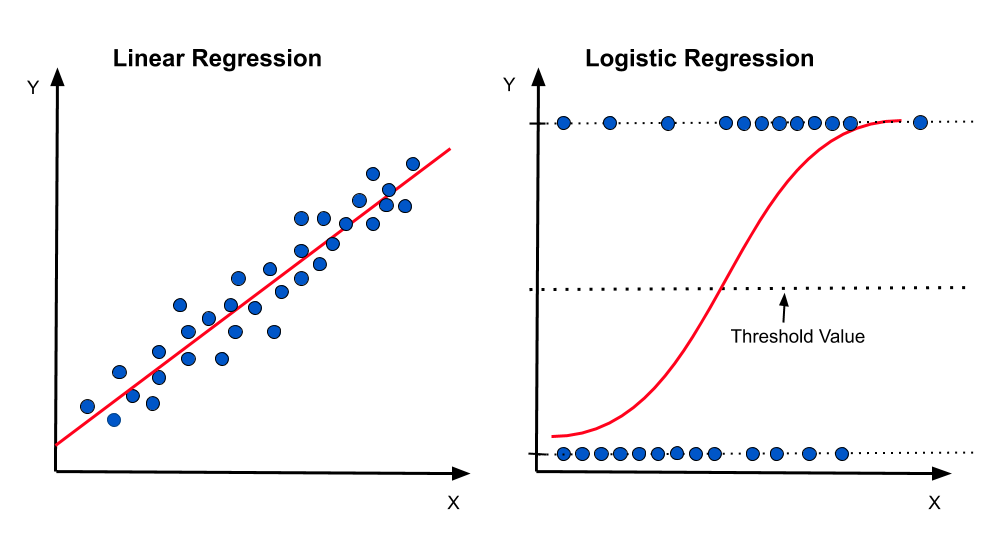
Linear Regression is a statistical method used to model the relationship between a dependent variable and one or more independent variables by fitting a linear equation to observed data. It assumes a linear relationship between the input features and the continuous target variable.
Logistic Regression, despite its name, is actually a classification algorithm that uses the logistic function to model the probability of binary or categorical outcomes. It transforms the linear combination of features using the sigmoid function to produce probabilities between 0 and 1.
The fundamental equation for Linear Regression is:
\[y = \beta_0 + \beta_1x_1 + \beta_2x_2 + ... + \beta_nx_n + \epsilon\]
The fundamental equation for Logistic Regression is:
\[P(y=1) = \frac{1}{1 + e^{-(\beta_0 + \beta_1x_1 + \beta_2x_2 + ... + \beta_nx_n)}}\]
When to Use Each Algorithm?
Use Linear Regression when:
- Your target variable is continuous (e.g., price, temperature, height)
- You want to predict numerical values
- The relationship between features and target appears linear
- You need to understand feature importance and interpretability
Use Logistic Regression when:
- Your target variable is categorical (binary or multinomial)
- You want to predict probabilities of class membership
- You need a probabilistic output for decision making
- You require model interpretability for classification tasks
| Aspect | Linear Regression | Logistic Regression |
|---|---|---|
| Problem Type | Regression | Classification |
| Output Variable | Continuous | Categorical (Probabilities) |
| Output Range | (-∞, +∞) | [0, 1] |
| Function Used | Linear Function | Sigmoid Function |
| Cost Function | Mean Squared Error | Log-Likelihood |
If you want to keep reading, I’ll now dive deeper into each strategy, then compare them, and finally explore some advanced strategies based on them.
2. Linear Regression Deep Dive
Mathematical Foundation of Linear Regression
Linear regression finds the best-fitting straight line through a set of data points by minimizing the sum of squared residuals. The mathematical foundation involves several key components:
Simple Linear Regression (One Feature):
\[y = \beta_0 + \beta_1x + \epsilon\]
Where:
- \(y\) = dependent variable (target)
- \(x\) = independent variable (feature)
- \(\beta_0\) = y-intercept
- \(\beta_1\) = slope (coefficient)
- \(\epsilon\) = error term
Multiple Linear Regression:
\[y = \beta_0 + \beta_1x_1 + \beta_2x_2 + \dots + \beta_nx_n + \epsilon\]
This equation extends simple linear regression to multiple features. It says that the predicted value \(y\) is given by an intercept \(\beta_0\) plus the sum of each feature \(x_j\) multiplied by its coefficient \(\beta_j\), and an error term \(\epsilon\) that captures noise or factors not explained by the model. Each coefficient \(\beta_j\) represents the average change in \(y\) when \(x_j\) increases by one unit, keeping all other variables fixed.
Matrix Form:
\[\mathbf{y} = \mathbf{X}\boldsymbol{\beta} + \boldsymbol{\epsilon}\]
This is the same model rewritten in compact matrix notation. Here, \(\mathbf{X}\) is a matrix where each row corresponds to one training example and each column to a feature, with the first column being all ones for the intercept term. Multiplying \(\mathbf{X}\) by the parameter vector \(\boldsymbol{\beta}\) produces all predicted values at once. The vector \(\boldsymbol{\epsilon}\) contains the residuals — the differences between actual outputs and predictions — for all \(m\) observations.
In matrix form:
- \(\mathbf{y}\): column vector of observed outputs (\(m \times 1\))
- \(\mathbf{X}\): design matrix of features with an intercept column (\(m \times (n+1)\))
- \(\boldsymbol{\beta}\): column vector of parameters (\((n+1) \times 1\))
- \(\boldsymbol{\epsilon}\): residuals vector (\(m \times 1\))
This compact representation makes it possible to apply linear algebra methods to solve for \(\boldsymbol{\beta}\) efficiently.
Cost Function (Mean Squared Error):
\[J(\boldsymbol{\beta}) = \frac{1}{2m} \sum_{i=1}^{m} \big( h_{\boldsymbol{\beta}}(x^{(i)}) - y^{(i)} \big)^2\]
The cost function measures how far the model’s predictions \(h_{\boldsymbol{\beta}}(x^{(i)})\) are from the actual outputs \(y^{(i)}\), by averaging the squared differences across all examples. The division by \(2m\) is used for convenience, as it simplifies derivative expressions in optimization. Minimizing \(J(\boldsymbol{\beta})\) finds the parameters that make predictions as close as possible to actual values in the least squares sense.
Assumptions of Linear Regression
Linear regression relies on several key assumptions. Violations can lead to unreliable predictions and misleading interpretations. The table below summarizes each assumption, its meaning, how to check it, and practical examples:
| Assumption | Description | How to Check | Example |
|---|---|---|---|
| Linearity |
The relationship between predictors and the target is linear. Model predicts a straight line or plane. |
Scatter plot of residuals vs. fitted values should show no
pattern. Residuals should be randomly scattered. |
Predicting house price from size: price increases proportionally
with size. If price jumps at certain sizes, linearity is violated. |
| Independence |
Observations are not related to each other. No autocorrelation in errors. |
Durbin-Watson test for autocorrelation. Time series: plot residuals over time. |
Predicting sales per store: each store's sales should not depend
on another's. If stores are in the same mall, independence may be violated. |
| Homoscedasticity |
Residuals have constant variance across all levels of
predictors. No "fanning out" or "funneling" in residuals. |
Residual plot: variance should be similar for all fitted
values. Look for equal spread. |
Predicting exam scores: error spread should be similar for low
and high scores. If errors increase for higher scores, assumption is violated. |
| Normality of Residuals |
Residuals are normally distributed. Important for valid confidence intervals and hypothesis tests. |
Q-Q plot of residuals. Histogram of residuals should look bell-shaped. |
Predicting height: residuals should cluster around zero. If residuals are skewed, normality is violated. |
| No Multicollinearity |
Predictors are not highly correlated with each other. High correlation makes coefficients unstable. |
Correlation matrix of predictors. Variance Inflation Factor (VIF) > 5-10 indicates a problem. |
Predicting salary from years of experience and age: if age and experience are highly correlated, multicollinearity exists. |
Step-by-Step Example: Normal Equation (Closed-form Solution)
\[\boldsymbol{\beta} = (\mathbf{X}^T\mathbf{X})^{-1}\mathbf{X}^T\mathbf{y}\]
Derived by setting the gradient of the cost function to zero, this equation gives the exact parameters that minimize the MSE without iterative optimization. It is efficient for problems with a small to moderate number of features, as it uses matrix operations to compute the optimal solution in one step.
Let's solve a simple regression problem step-by-step using the normal equation. Suppose we have 3 training examples with 1 feature (\(x_1\)) and an intercept:
\[ \mathbf{X} = \begin{bmatrix} 1 & 1 \\ 1 & 2 \\ 1 & 3 \end{bmatrix} \quad (3 \times 2), \quad \mathbf{y} = \begin{bmatrix} 1 \\ 2 \\ 2 \end{bmatrix} \quad (3 \times 1) \]
Step 1 – Compute \( \mathbf{X}^T \mathbf{X} \)
\[ \mathbf{X}^T = \begin{bmatrix} 1 & 1 & 1 \\ 1 & 2 & 3 \end{bmatrix} \quad (2 \times 3) \]
\[ \mathbf{X}^T \mathbf{X} = \begin{bmatrix} 1 & 1 & 1 \\ 1 & 2 & 3 \end{bmatrix} \begin{bmatrix} 1 & 1 \\ 1 & 2 \\ 1 & 3 \end{bmatrix} = \begin{bmatrix} 3 & 6 \\ 6 & 14 \end{bmatrix} \quad (2 \times 2) \]
Step 2 – Compute \( (\mathbf{X}^T \mathbf{X})^{-1} \)
Determinant: \[ \det = (3)(14) - (6)(6) = 42 - 36 = 6 \]
Inverse:
\[ (\mathbf{X}^T \mathbf{X})^{-1} = \frac{1}{6} \begin{bmatrix} 14 & -6 \\ -6 & 3 \end{bmatrix} = \begin{bmatrix} 2.333\ldots & -1 \\ -1 & 0.5 \end{bmatrix} \]
Step 3 – Compute \( \mathbf{X}^T \mathbf{y} \)
\[ \mathbf{X}^T \mathbf{y} = \begin{bmatrix} 1 & 1 & 1 \\ 1 & 2 & 3 \end{bmatrix} \begin{bmatrix} 1 \\ 2 \\ 2 \end{bmatrix} = \begin{bmatrix} 5 \\ 11 \end{bmatrix} \]
Step 4 – Multiply to find \( \boldsymbol{\beta} \)
\[ \boldsymbol{\beta} = \begin{bmatrix} 2.333\ldots & -1 \\ -1 & 0.5 \end{bmatrix} \begin{bmatrix} 5 \\ 11 \end{bmatrix} = \begin{bmatrix} 11.666\ldots - 11 \\ -5 + 5.5 \end{bmatrix} = \begin{bmatrix} 0.666\ldots \\ 0.5 \end{bmatrix} \]
Step 5 – Final model
Estimated coefficients: \[ \beta_0 \approx 0.667, \quad \beta_1 = 0.5 \]
Final equation: \[ \hat{y} = 0.667 + 0.5 x_1 \]
Interpretation: when \(x_1\) increases by 1, the predicted \(y\) increases by 0.5 on average, starting from a baseline of about 0.667.
Step-by-Step Example: Gradient Descent
While the Normal Equation provides an exact solution, Gradient Descent offers an iterative approach that's more scalable for large datasets. Let's apply it to the same toy example to compare both methods.
We will use the same dataset as before, with 3 training examples and 1 feature (\(x_1\)). Here's the python code:
Convergence Analysis
The gradient descent algorithm iteratively updates the parameters using the formula:
\[\boldsymbol{\beta}^{(t+1)} = \boldsymbol{\beta}^{(t)} - \alpha \nabla J(\boldsymbol{\beta}^{(t)})\]
where \(\alpha\) is the learning rate and \(\nabla J\) is the gradient of the cost function.
Gradient Descent Results (α = 0.1, 500 iterations)
| Iteration | β₀ | β₁ | Cost J(β) |
|---|---|---|---|
| 0 | 0.000000 | 0.000000 | 1.500000 |
| 1 | 0.166667 | 0.366667 | 0.327593 |
| 2 | 0.243333 | 0.528889 | 0.094871 |
| 5 | 0.309218 | 0.643345 | 0.037130 |
| 10 | 0.334922 | 0.645692 | 0.035668 |
| 50 | 0.462202 | 0.589945 | 0.030776 |
| 100 | 0.554972 | 0.549135 | 0.028673 |
| 250 | 0.648458 | 0.508010 | 0.027802 |
| 500 | 0.665781 | 0.500390 | 0.027778 |
Gradient Descent Results (α = 0.01, 10,000 iterations)
| Iteration | β₀ | β₁ | Cost J(β) |
|---|---|---|---|
| 0 | 0.000000 | 0.000000 | 1.500000 |
| 1 | 0.016667 | 0.036667 | 1.342276 |
| 2 | 0.032433 | 0.071289 | 1.201560 |
| 5 | 0.074819 | 0.163992 | 0.864088 |
| 10 | 0.131609 | 0.287039 | 0.504637 |
| 50 | 0.297364 | 0.616713 | 0.041550 |
| 100 | 0.333821 | 0.643781 | 0.035694 |
| 1000 | 0.554236 | 0.549458 | 0.028684 |
| 5000 | 0.665751 | 0.500403 | 0.027778 |
| 10000 | 0.666664 | 0.500001 | 0.027778 |
Method Comparison
| Method | β₀ | β₁ | Final Cost | Iterations |
|---|---|---|---|---|
| Normal Equation | 0.666667 | 0.500000 | 0.027777777778 | N/A (closed-form) |
| Gradient Descent (α=0.1) | 0.665781 | 0.500390 | 0.027777834064 | 500 |
| Gradient Descent (α=0.01) | 0.666664 | 0.500001 | 0.027777777778 | 10,000 |
The same results were achieved using different methods.
Key Insights
Normal Equation
- Pros:
- Instant exact solution
- No hyperparameters to tune
- Guaranteed global minimum
- Cons:
- O(n³) complexity (matrix inversion)
- Memory intensive for large datasets
- Not suitable when n > 10,000
Gradient Descent
- Pros:
- O(mn) per iteration
- Works with huge datasets
- Memory efficient
- Cons:
- Requires many iterations
- Learning rate tuning needed
- May converge to local minimum
Evaluation Metrics for Linear Regression
Evaluating linear regression models requires metrics that quantify how well the model predicts the target variable. The table below summarizes common metrics, their formulas, and when to use them:
| Metric | Formula | Description |
|---|---|---|
| Mean Squared Error (MSE) | \[MSE = \frac{1}{m}\sum_{i=1}^{m}(y_i - \hat{y}_i)^2\] |
Average squared difference between actual and predicted
values. Use it when: Penalizing larger errors is important, useful for model optimization. Don't use it when: Data has outliers or you need more interpretable error units. |
| Root Mean Squared Error (RMSE) | \[RMSE = \sqrt{\frac{1}{m}\sum_{i=1}^{m}(y_i - \hat{y}_i)^2}\] |
Square root of MSE, interpretable in original units. Use it when: You want error in the same units as the target variable. Don't use it when: Outliers dominate or you need error direction. |
| Mean Absolute Error (MAE) | \[MAE = \frac{1}{m}\sum_{i=1}^{m}|y_i - \hat{y}_i|\] |
Average absolute difference between actual and predicted
values. Use it when: You want a direct error measure and less sensitivity to outliers. Don't use it when: Penalizing large errors is critical or for optimization. |
| R-squared (R²) | \[R^2 = 1 - \frac{\sum_{i=1}^{m}(y_i - \hat{y}_i)^2}{\sum_{i=1}^{m}(y_i - \bar{y})^2}\] |
Proportion of variance explained by the model. Use it when: Assessing overall model fit and explanatory power. Don't use it when: Model is non-linear or has many predictors; does not indicate overfitting. |
| Adjusted R-squared | \[R^2_{adj} = 1 - \frac{(1-R^2)(m-1)}{m-p-1}\] |
R² adjusted for number of predictors (\(m\): samples, \(p\):
predictors). Use it when: Comparing models with different numbers of predictors. Don't use it when: Interpretation needs to be intuitive or predictors are irrelevant. |
3. Logistic Regression Deep Dive
Mathematical Foundation of Logistic Regression
Logistic regression uses the sigmoid (logistic) function to map any real-valued input to a value between 0 and 1, making it perfect for probability estimation and binary classification.
Sigmoid Function:
\[\sigma(z) = \frac{1}{1 + e^{-z}}\]
The sigmoid (or logistic) function maps any real-valued input \(z\) into the range \((0, 1)\), making it ideal for modeling probabilities. When \(z\) is large and positive, \(\sigma(z) \approx 1\); when \(z\) is large and negative, \(\sigma(z) \approx 0\); and when \(z = 0\), the output is exactly \(0.5\). Its smooth, S-shaped curve ensures small changes in \(z\) near zero cause significant changes in \(\sigma(z)\), which is useful for classification.
Linear Combination:
\[z = \beta_0 + \beta_1x_1 + \beta_2x_2 + \dots + \beta_nx_n\]
This is the weighted sum of input features used in logistic regression. Each feature \(x_j\) is multiplied by its corresponding coefficient \(\beta_j\), and \(\beta_0\) is the intercept (bias term). The value \(z\) is not yet constrained between 0 and 1 — it can be any real number — and will be passed through the sigmoid function to obtain a probability.
Probability of Positive Class:
\[P(y=1 \mid x) = \frac{1}{1 + e^{-(\beta_0 + \beta_1x_1 + \dots + \beta_nx_n)}}\]
This applies the sigmoid function to the linear combination \(z\) to get the probability that the output class \(y\) equals 1, given the features \(x\). The exponent term flips sign depending on the direction of \(z\), producing probabilities near 1 when \(z\) is strongly positive and near 0 when \(z\) is strongly negative.
Odds and Log-Odds:
The odds of an event is the ratio between the probability of the event occurring and the probability of it not occurring:
\[Odds = \frac{P(y=1)}{P(y=0)} = \frac{P(y=1)}{1 - P(y=1)}\]
If \(P(y=1)\) is 0.75, the odds are \(0.75 / 0.25 = 3\), meaning the event is three times as likely to happen than not.
Taking the natural logarithm of the odds gives the log-odds (logit), which in logistic regression is a linear function of the input:
\[\text{logit}(p) = \ln\left(\frac{p}{1-p}\right) = \beta_0 + \beta_1x_1 + \dots + \beta_nx_n\]
This equation shows that while probabilities themselves are not linear in the inputs, their log-odds are — making the model suitable for estimation with linear methods while still producing probabilistic outputs.
This shows that logistic regression is actually modeling the log-odds as a linear function of the features.
Maximum Likelihood Estimation
Unlike linear regression, logistic regression doesn't have a closed-form solution. Instead, it uses Maximum Likelihood Estimation (MLE) to find the optimal parameters. This means we look for the values of \(\boldsymbol{\beta}\) that make the observed training data most probable.
Likelihood Function:
For a binary classification problem, the likelihood of observing the data given the parameters is:
\[L(\boldsymbol{\beta}) = \prod_{i=1}^{m} P(y^{(i)} \mid x^{(i)};\boldsymbol{\beta})\]
This formula says the likelihood \( L(\boldsymbol{\beta}) \) is the product, over all \( m \) training examples, of the predicted probability of the actual observed class. If \( y^{(i)} = 1 \), the term is \( h_{\boldsymbol{\beta}}(x^{(i)}) \); if \( y^{(i)} = 0 \), it is \( 1 - h_{\boldsymbol{\beta}}(x^{(i)}) \). Multiplying these terms gives the joint probability of the dataset under the model.
Log-Likelihood Function:
Taking the logarithm makes the optimization easier:
\[\ell(\boldsymbol{\beta}) = \sum_{i=1}^{m} \left[ y^{(i)} \log(h_{\boldsymbol{\beta}}(x^{(i)})) + (1-y^{(i)})\log(1-h_{\boldsymbol{\beta}}(x^{(i)})) \right]\]
The log transforms the product into a sum, helping numerical stability and simplifying derivatives. When \( y^{(i)} = 1 \), only the first log term remains; when \( y^{(i)} = 0 \), only the second term remains. Adding these over all samples yields the log-probability of the data given \(\boldsymbol{\beta}\).
Cost Function (Negative Log-Likelihood):
\[J(\boldsymbol{\beta}) = -\frac{1}{m} \sum_{i=1}^{m} \left[ y^{(i)}\log(h_{\boldsymbol{\beta}}(x^{(i)})) + (1-y^{(i)})\log(1-h_{\boldsymbol{\beta}}(x^{(i)})) \right]\]
Maximizing the log-likelihood is equivalent to minimizing the negative log-likelihood. This is our cost function. The minus sign converts the maximization problem into a minimization problem suitable for gradient descent, and dividing by \( m \) gives the average cost per training example.
Gradient Descent Update:
The parameters are updated using gradient descent:
\[\beta_j := \beta_j - \alpha \frac{\partial J(\boldsymbol{\beta})}{\partial \beta_j}\]
Starting from initial values, each parameter \(\beta_j\) is adjusted in the opposite direction of the gradient of the cost function to reduce it. Here, \(\alpha\) is the learning rate, controlling step size.
Where the gradient is:
\[\frac{\partial J(\boldsymbol{\beta})}{\partial \beta_j} = \frac{1}{m}\sum_{i=1}^{m} \left( h_{\boldsymbol{\beta}}(x^{(i)}) - y^{(i)} \right) x_j^{(i)}\]
This derivative measures the average prediction error \((h_{\boldsymbol{\beta}}(x^{(i)}) - y^{(i)})\) multiplied by the \( j^{th} \) feature value \( x_j^{(i)} \). If the predictions are perfect, the gradient becomes zero and the parameters stop changing.
Step-by-Step Example: Logistic Regression with Gradient Descent
Let's walk through a simple logistic regression example to illustrate how the algorithm works in practice.
Problem: Predict whether a student passes (1) or fails (0) an exam based on the number of hours studied.
Dataset:
| Hours Studied | Pass (1) / Fail (0) |
|---|---|
| 1 | 0 |
| 2 | 0 |
| 3 | 0 |
| 4 | 1 |
| 5 | 1 |
| 6 | 1 |
| 7 | 1 |
Step 1 – Set up the logistic regression model
Define the mathematical relationship between the input feature and the probability of a positive outcome using the sigmoid function.
The logistic regression probability model is:
\[ P(y=1|x) = \frac{1}{1 + e^{-(\beta_0 + \beta_1 x)}} \]
- \(x\) = hours studied (input feature)
- \(y\) = pass/fail (target)
- \(\beta_0\) = intercept
- \(\beta_1\) = coefficient
Step 2 – Initialize parameters
Begin the learning process by assigning initial guess values to the model’s parameters.
Example initial values:
\[ \beta_0 = 0, \quad \beta_1 = 0 \]
Step 3 – Compute predictions
Use the current parameters to calculate the predicted probability of passing for each training example using the sigmoid function.
Example for \(x = 4\) hours studied:
\[ z = \beta_0 + \beta_1 \times 4 \] \[ P(y=1|x=4) = \frac{1}{1 + e^{-z}} \]
Step 4 – Calculate the cost (log-loss)
Measure how far the predictions are from the actual target values using the log-loss function.
The cost function is:
\[ J(\beta_0, \beta_1) = -\frac{1}{m} \sum_{i=1}^{m} \left[ y^{(i)}\log(p^{(i)}) + (1-y^{(i)})\log(1-p^{(i)}) \right] \]
Step 5 – Update parameters using gradient descent
Adjust the model parameters in the direction that reduces the cost, using the calculated gradients.
Gradient descent update rule:
\[ \beta_j := \beta_j - \alpha \frac{\partial J}{\partial \beta_j} \]
- Repeat Steps 3–5 until convergence (when cost stops decreasing).
Step 6 – Make predictions (after training)
Use the optimized parameters to estimate the probability of passing for new data points.
Suppose after training we have:
\[ \beta_0 = -6, \quad \beta_1 = 1.2 \]
For \(x = 5\) hours:
\[ z = -6 + 1.2 \times 5 = 0 \] \[ P(y=1|x=5) = \frac{1}{1 + e^{0}} = 0.5 \]
For \(x = 7\) hours:
\[ z = -6 + 1.2 \times 7 = 2.4 \] \[ P(y=1|x=7) = \frac{1}{1 + e^{-2.4}} \approx 0.916 \]
Step 7 – Classification rule
Convert predicted probabilities into binary outcomes based on a decision threshold.
If \(P(y=1|x) > 0.5\), predict "pass" (1); otherwise, predict "fail" (0).
This step-by-step process demonstrates how logistic regression models the probability of a binary outcome and makes decisions based on a chosen threshold.
Evaluation Metrics for Logistic Regression
| Metric | Formula | Description |
|---|---|---|
| Accuracy | \[Accuracy = \frac{TP + TN}{TP + TN + FP + FN}\] |
Proportion of correct predictions. Use it when: Dataset is balanced and all errors are equally important. Don't use it when: Classes are imbalanced. |
| Precision | \[Precision = \frac{TP}{TP + FP}\] |
Fraction of predicted positives that are correct. Use it when: False positives are costly (e.g., spam detection). Don't use it when: False negatives matter more. |
| Recall (Sensitivity) | \[Recall = \frac{TP}{TP + FN}\] |
Fraction of actual positives detected. Use it when: Missing positives is costly (e.g., disease detection). Don't use it when: False positives matter more. |
| F1-Score | \[F1 = 2 \times \frac{Precision \times Recall}{Precision + Recall}\] |
Harmonic mean of precision and recall. Use it when: Data is imbalanced and you want a balance between precision and recall. Don't use it when: You need a metric that's easy to interpret or when classes are balanced. |
| ROC-AUC | \[ROC\text{-}AUC = \int_{0}^{1} TPR(FPR) \, dFPR\] |
Measures ability to distinguish classes. Consider: TPR (True Positive Rate): \(TPR = \frac{TP}{TP + FN}\) — proportion of actual positives correctly identified. FPR (False Positive Rate): \(FPR = \frac{FP}{FP + TN}\) — proportion of actual negatives incorrectly identified as positive. Use it when: You want a threshold-independent metric for ranking models. Don't use it when: Practical decision thresholds are more important. |
| Log-Loss | \[Log Loss = -\frac{1}{m}\sum_{i=1}^{m} [y_i\log(p_i) + (1-y_i)\log(1-p_i)]\] |
Penalizes confident wrong predictions. Use it when: You care about probability calibration and penalizing overconfident errors. Don't use it when: You want a simple, interpretable metric. |
4. Detailed Comparison
Understanding the fundamental differences between linear and logistic regression is crucial for choosing the right algorithm for your specific problem. This comprehensive comparison examines mathematical foundations, practical considerations, and performance characteristics.
Mathematical Foundations Comparison
Hypothesis Functions and Transformations
Linear Regression
Interpretation: Direct linear combination of features. The output is unbounded and represents the predicted continuous value.
Mathematical Nature: Linear function mapping features to real-valued outputs.
Logistic Regression
Interpretation: Linear combination passed through sigmoid function. Output represents probability of positive class.
Mathematical Nature: Non-linear function (due to sigmoid) mapping features to probabilities [0,1].
While both use linear combinations of features, logistic regression applies a non-linear transformation (sigmoid) that fundamentally changes the problem from regression to classification.
Output Characteristics and Interpretation
| Characteristic | Linear Regression | Logistic Regression | Practical Implication |
|---|---|---|---|
| Output Range | (-∞, +∞) | (0, 1) | Linear can predict any value; Logistic bounded to probabilities |
| Output Type | Continuous numerical value | Probability/likelihood | Different interpretation and use cases |
| Threshold | Not applicable | Typically 0.5 for binary decisions | Logistic requires decision threshold for classification |
| Confidence | Prediction intervals | Probability scores | Different ways to express uncertainty |
Cost Functions and Optimization
Linear Regression Cost Function
Properties:
- Convex function (single global minimum)
- Quadratic in parameters
- Sensitive to outliers (squared error)
- Has closed-form solution (Normal Equation)
Logistic Regression Cost Function
Properties:
- Convex function (due to log-concave likelihood)
- Logarithmic penalty structure
- More robust to outliers
- No closed-form solution (requires iterative methods)
Why Different Cost Functions?
Linear regression uses MSE because it's the maximum likelihood estimator under Gaussian noise assumptions. Logistic regression uses cross-entropy because it's the negative log-likelihood of the Bernoulli distribution, making it the natural choice for binary classification problems.
Parameter Estimation Methods
| Method | Linear Regression | Logistic Regression | Computational Complexity |
|---|---|---|---|
| Closed-form Solution | ✓ Normal Equation: \(\boldsymbol{\theta} = (X^TX)^{-1}X^Ty\) | ✗ No closed-form solution | O(n³) for matrix inversion |
| Gradient Descent | ✓ Optional (useful for large datasets) | ✓ Required method | O(mn) per iteration |
| Newton's Method | ✓ Rarely used (MSE is quadratic) | ✓ Often used (Newton-Raphson) | O(n³) per iteration (Hessian) |
| Convergence | One-step (Normal Eq.) or linear convergence | Quadratic convergence (Newton's method) | Varies by method |
Decision Boundaries and Geometric Interpretation
Linear Regression
Geometric Interpretation: Finds the best-fitting hyperplane that minimizes perpendicular distances to data points.
Decision Boundary: No explicit boundary - it's a regression task. If forced into classification (threshold at some value), creates a linear boundary.
Margin Concept: Not applicable - focuses on minimizing prediction error.
Logistic Regression
Geometric Interpretation: Creates a linear decision boundary in feature space where \(P(y=1|x) = 0.5\).
Decision Boundary: Explicitly defined where \(\boldsymbol{\theta}^T x = 0\). Points on one side have \(P > 0.5\), others have \(P < 0.5\).
Margin Concept: Soft margin - probability gradually changes across the boundary.
\[\boldsymbol{\theta}^T x = 0 \Rightarrow \theta_0 + \theta_1x_1 + ... + \theta_nx_n = 0\]
This hyperplane separates the feature space into regions of different class predictions.
Comprehensive Assumptions Analysis
| Assumption | Linear Regression | Logistic Regression | Violation Consequences | Diagnostic Methods |
|---|---|---|---|---|
| Linearity | Linear relationship between X and Y | Linear relationship between X and log-odds | Biased estimates, poor predictions | Residual plots, scatter plots |
| Independence | Observations must be independent | Observations must be independent | Underestimated standard errors | Durbin-Watson test, ACF plots |
| Normality | Residuals should be normal | Not required | Invalid confidence intervals | Q-Q plots, Shapiro-Wilk test |
| Homoscedasticity | Constant variance of residuals | Not strictly required | Inefficient estimates, wrong SEs | Breusch-Pagan test, residual plots |
| No Multicollinearity | Features should not be highly correlated | Features should not be highly correlated | Unstable coefficients, inflated SEs | VIF, correlation matrix |
| Sample Size | At least 10-15 obs per predictor | At least 10-20 events per predictor | Overfitting, unreliable estimates | Power analysis, cross-validation |
| No Perfect Separation | Not applicable | No feature perfectly separates classes | Non-convergence, infinite coefficients | Check for separation, regularization |
Performance Characteristics and Trade-offs
Computational Efficiency
| Aspect | Linear Regression | Logistic Regression | Practical Impact |
|---|---|---|---|
| Training Time | O(n³) normal equation, O(mn) gradient descent | O(mn×iterations) gradient descent | Linear often faster for small datasets |
| Prediction Time | O(n) - simple dot product | O(n) - dot product + sigmoid | Nearly identical in practice |
| Memory Usage | Stores coefficient vector | Stores coefficient vector | Identical memory requirements |
| Scalability | Excellent for large datasets | Good, requires iterative training | Both scale well with modern optimizers |
Robustness and Sensitivity Analysis
Linear Regression Robustness
Outlier Sensitivity: High - squared error amplifies outliers
Feature Scaling: Not required for basic algorithm, but recommended for gradient descent
Missing Data: Requires complete cases or imputation
Noise Tolerance: Moderate - Gaussian noise assumption
Logistic Regression Robustness
Outlier Sensitivity: Lower - logarithmic cost function is more robust
Feature Scaling: Highly recommended for proper convergence
Missing Data: Requires complete cases or imputation
Noise Tolerance: Good - no distributional assumptions on features
Advantages and Limitations
Linear Regression: Detailed Analysis
Unique Advantages:
- Interpretability: Coefficients directly represent marginal effects
- Prediction Intervals: Can provide confidence bounds for predictions
- Statistical Testing: Rich framework for hypothesis testing (t-tests, F-tests)
- Extrapolation: Can reasonably extrapolate beyond training data range
- Feature Importance: Coefficient magnitude indicates feature importance
- Simplicity: Easy to implement, debug, and explain to stakeholders
Critical Limitations:
- Linearity Assumption: Cannot capture non-linear relationships without feature engineering
- Outlier Vulnerability: Single extreme points can skew entire model
- Heteroscedasticity Issues: Violates assumptions when error variance changes
- Multicollinearity Problems: Unstable coefficients with correlated features
- Distribution Sensitivity: Assumes Gaussian errors for inference
- Limited Flexibility: Cannot handle categorical targets or complex patterns
Logistic Regression: Detailed Analysis
Unique Advantages:
- Probabilistic Output: Provides uncertainty quantification via probabilities
- No Distributional Assumptions: More flexible regarding data distributions
- Outlier Resistance: Logarithmic loss is less sensitive to extreme values
- Natural Classification: Designed specifically for categorical outcomes
- Interpretable Odds Ratios: Coefficients represent log-odds ratios
- Extension to Multi-class: Naturally extends to multinomial classification
- Regularization Friendly: Works well with L1/L2 regularization
Critical Limitations:
- Linear Decision Boundary: Cannot capture complex non-linear separations
- Sample Size Requirements: Needs large samples for stable estimates
- Perfect Separation Issues: Fails when classes are perfectly separable
- Feature Scaling Dependency: Requires careful preprocessing for optimal performance
- Convergence Challenges: May not converge with poorly conditioned data
- Limited Extrapolation: Probabilities can become extreme outside training range
5. Practical Considerations
Successfully implementing linear and logistic regression requires moving beyond theory into careful data preparation, feature engineering, and rigorous model validation. This section provides a comprehensive guide to the practical steps that distinguish a mediocre model from a high-performing, reliable one.
Data Preprocessing Pipeline
Essential Preprocessing Steps for Both Algorithms
Step 1: Data Quality Assessment
Missing Values Analysis: Before imputation, diagnose the mechanism of missingness. Is it Missing Completely At Random (MCAR), where there's no pattern? Missing At Random (MAR), where missingness depends on other observed features? Or Missing Not At Random (MNAR), where it depends on the missing value itself? The mechanism dictates valid handling strategies and potential biases.
Outlier Detection: Use statistical methods (IQR, Z-score) and robust techniques (Isolation Forest) alongside visualization (box plots, scatter plots) to identify extreme values. Outliers can disproportionately influence coefficient estimates in linear regression and decision boundaries in logistic regression.
Data Distribution Analysis: Analyze the skewness and kurtosis of each feature and the target variable. This informs decisions on transformations (e.g., log, Box-Cox) needed to meet model assumptions or improve performance.
Step 2: Feature Scaling and Normalization
Why It Matters: Essential for models using gradient descent or regularization. Without scaling, features with larger numeric ranges can dominate the cost function, leading to slow convergence and preventing regularization from working as intended, as the penalty term would be unevenly applied.
When to Apply: Critical for logistic regression and any linear regression solved with gradient descent or regularization (Ridge, Lasso, Elastic Net). Less critical for simple linear regression with an analytical solution (Normal Equation), but still good practice.
Methods: Use StandardScaler (for algorithms assuming a normal distribution), MinMaxScaler (when you need a fixed [0, 1] range), or RobustScaler (when dealing with significant outliers, as it uses the interquartile range).
Step 3: Missing Value Handling
Numerical Features: Simple methods include mean/median/mode imputation. More advanced approaches like K-Nearest Neighbors (KNN) imputation or model-based imputation (e.g., using a regression model to predict the missing value) can capture relationships in the data more effectively.
Categorical Features: Impute with the mode, create a dedicated "Missing" category to capture potential information in the missingness itself, or use domain knowledge.
Advanced Approach: Use Multiple Imputation by Chained Equations (MICE), which creates multiple complete datasets, runs the model on each, and pools the results. This properly accounts for the uncertainty introduced by imputation.
Algorithm-Specific Preprocessing Requirements
Linear Regression Preprocessing
Linearity Enhancement:
- Polynomial Features: Add \(x^2, x^3\) to model non-linear relationships.
- Interaction Terms: Create \(x_1 \times x_2\) to capture synergistic effects where the impact of one feature depends on the level of another.
- Log & Box-Cox Transformations: Apply to features or the target to stabilize variance (homoscedasticity), normalize distributions, and linearize exponential relationships.
Assumption Validation:
- Linearity: Check with residual vs. fitted plots; a random scatter around zero is ideal.
- Homoscedasticity (Constant Variance): Test with Breusch-Pagan test or by observing the spread in the residual vs. fitted plot.
- Normality of Residuals: Verify with Q-Q plots; points should follow the diagonal line.
- Multicollinearity: Detect with Variance Inflation Factor (VIF) scores. A VIF > 5 or 10 indicates that a feature is highly correlated with others, which can destabilize coefficient estimates.
Logistic Regression Preprocessing
Categorical Handling:
- One-Hot Encoding: Creates binary columns for nominal features. Best for low-cardinality variables to avoid the "curse of dimensionality."
- Ordinal Encoding: Maps ordered categories to integers (e.g., "low," "medium," "high" to 0, 1, 2).
- Target Encoding: Replaces a category with the mean of the target variable. Powerful but carries a high risk of data leakage; requires careful implementation within a cross-validation loop.
Class Balance Management:
- Class Weights: Adjust the model's cost function to more heavily penalize errors on the minority class.
- Oversampling (e.g., SMOTE): Creates synthetic examples of the minority class. Best when data is limited.
- Undersampling: Removes examples from the majority class. Useful for very large datasets but risks discarding important information.
- Evaluation: Always use metrics like Precision, Recall, F1-Score, or AUC-PR that are robust to class imbalance.
Advanced Feature Engineering Techniques
Domain-Specific Feature Creation
Time-Based Features: From a timestamp, create features like day of the week, month, is_holiday, time since last event, or rolling averages/standard deviations over a time window to capture trends and seasonality.
Text Features: Transform unstructured text into meaningful numbers using TF-IDF vectors, pre-trained word embeddings (e.g., Word2Vec, GloVe), sentiment scores, or engineered metrics like text length or keyword counts.
Geospatial Features: From latitude/longitude, calculate distances between points, cluster locations, or enrich data with external sources like population density, weather patterns, or proximity to points of interest.
Model Validation and Selection Strategies
Cross-Validation Methodologies
Standard Cross-Validation
K-Fold Cross-Validation: The default choice (k=5 or 10). Provides a robust estimate of model performance by training and testing on different subsets of the data.
Stratified K-Fold: Essential for imbalanced classification. Ensures that the class distribution in each fold mirrors the overall dataset, preventing folds with zero minority class samples.
Specialized Validation
Time Series Split: Critically important for temporal data to prevent data leakage from the future. The training set always precedes the test set (e.g., train on years 1-3, test on year 4).
Group K-Fold: Use when data has non-independent groups (e.g., multiple readings from the same patient). Ensures that all data from one group is in either the training or the test set, never split across both.
Nested CV: The gold standard for reporting performance. An outer loop splits data for evaluation, and an inner loop performs hyperparameter tuning on the training portion only, providing an unbiased performance estimate.
Regularization Techniques
Regularization adds a penalty to the cost function based on the size of the coefficients, preventing overfitting and improving generalization.
\[J(\boldsymbol{\beta}) = \text{Cost} + \lambda\sum_{j=1}^{n}\beta_j^2\]
Shrinks coefficients toward zero but rarely to exactly zero. Excellent for handling multicollinearity and when you believe many features are relevant.
\[J(\boldsymbol{\beta}) = \text{Cost} + \lambda\sum_{j=1}^{n}|\beta_j|\]
Can shrink coefficients to exactly zero, performing automatic feature selection. Ideal for creating sparse, interpretable models when you suspect many features are irrelevant.
\[J(\boldsymbol{\beta}) = \text{Cost} + \lambda_1\sum_{j=1}^{n}|\beta_j| + \lambda_2\sum_{j=1}^{n}\beta_j^2\]
A hybrid that combines the strengths of both. It can perform feature selection like Lasso but is more stable in the presence of highly correlated features, where it tends to group and shrink their coefficients together.
Hyperparameter Tuning Strategies
Grid Search: An exhaustive search over a manually specified grid of hyperparameters. Guaranteed to find the best combination within the grid but is computationally expensive.
Random Search: Samples a fixed number of combinations from a statistical distribution. More efficient than grid search, especially for high-dimensional spaces where some hyperparameters are more important than others.
Bayesian Optimization: An intelligent search method that uses a probabilistic model to decide which hyperparameter combination to try next based on past results. Balances exploration and exploitation to find optimal values in fewer iterations.
Performance Optimization and Diagnostics
Computational Efficiency Considerations
| Aspect | Linear Regression | Logistic Regression | Optimization Tips |
|---|---|---|---|
| Solvers | Normal Equation (exact, fast for small N features) or Gradient Descent (iterative, scales to large N). | Iterative solvers only (e.g., liblinear, saga, lbfgs). | Choose a solver based on dataset size; 'saga' is often a good default for large datasets with regularization. |
| Large Datasets | Use Stochastic Gradient Descent (SGD) for out-of-core learning. | Use mini-batch gradient descent for a balance of speed and stability. | Process data in chunks if it doesn't fit in memory. |
Model Diagnostics and Debugging
Linear Regression Diagnostics
Residual Analysis:
- Residuals vs. Fitted Plot: Look for non-linear patterns (e.g., a curve) or non-constant variance (e.g., a funnel shape).
- Cook's Distance: Identify influential points that, if removed, would significantly change the model's coefficients.
Model Quality Metrics:
- R² vs. Adjusted R²: Adjusted R² penalizes the addition of useless features, making it better for comparing models with different numbers of predictors.
- RMSE/MAE: Provide error magnitude in the original units of the target, making them easy to interpret.
Logistic Regression Diagnostics
Classification Performance:
- Confusion Matrix: The foundation for calculating Precision, Recall, and F1-score.
- ROC vs. Precision-Recall Curves: Use ROC curves for balanced datasets and PR curves for imbalanced datasets to evaluate trade-offs.
- Calibration Plot: Checks if the predicted probabilities are reliable (e.g., if for all predictions of 0.8, 80% of them are actually positive).
Model Interpretation:
- Odds Ratios: Interpret coefficients by converting them to odds ratios (\(e^\beta\)). An odds ratio of 1.2 means a one-unit increase in the feature increases the odds of the positive class by 20%.
- SHAP/LIME: Use these model-agnostic methods to explain individual predictions, providing local, instance-level interpretability.
6. Implementation Examples
Linear Regression: From Scratch Implementation
Understanding linear regression requires implementing it from first principles. This implementation demonstrates the mathematical concepts in practice.
Logistic Regression: From Scratch Implementation
Logistic regression implementation from scratch demonstrates the sigmoid function, maximum likelihood estimation, and gradient descent optimization.
Advanced Topics and Extensions
Polynomial Regression: Mathematical Foundation
Polynomial regression extends linear regression by adding polynomial terms of the features (e.g., squared, cubed) to the model. This transformation allows the model to fit non-linear patterns in the data while still leveraging the efficient estimation techniques of linear regression.
Mathematical Formulation:
For a single feature, a polynomial regression of degree \(d\) is defined as:
\[y = \beta_0 + \beta_1x + \beta_2x^2 + \beta_3x^3 + \dots + \beta_dx^d + \epsilon\]
This equation models the target \(y\) as a \(d\)-degree polynomial function of the feature \(x\). The model learns coefficients \(\beta_j\) for each power of \(x\), allowing it to fit curves instead of just straight lines. The \(\epsilon\) term represents the irreducible error.
For multiple features, the model also includes interaction terms:
\[y = \beta_0 + \sum_{i=1}^{n}\beta_i x_i + \sum_{i=1}^{n}\sum_{j=i}^{n}\beta_{ij}x_i x_j + \dots + \epsilon\]
This form captures not only the polynomial effect of each feature (e.g., \(x_1^2\)) but also how features interact with each other (e.g., \(x_1x_2\)). This allows the model to fit complex, multi-dimensional surfaces.
Feature Transformation:
The core idea is to transform the original feature set into a new, higher-dimensional one that includes the polynomial terms. Polynomial regression is fundamentally a linear regression model applied to these transformed features.
\[\mathbf{X}_{\text{poly}} = [1, x_1, x_2, \dots, x_n, x_1^2, x_1x_2, \dots, x_n^2, x_1^3, \dots]\]
We create a new feature matrix, \(\mathbf{X}_{\text{poly}}\), where each row corresponds to an observation and each column represents a term in the polynomial expansion (e.g., \(x_1\), \(x_1^2\), \(x_1x_2\)).
Matrix Form:
Using the transformed features, the model is expressed in a familiar linear form:
\[\mathbf{y} = \mathbf{X}_{\text{poly}}\boldsymbol{\beta} + \boldsymbol{\epsilon}\]
This equation is identical in structure to multiple linear regression. The vector \(\mathbf{y}\) contains the target values, \(\mathbf{X}_{\text{poly}}\) is the transformed feature matrix, \(\boldsymbol{\beta}\) is the vector of coefficients to be learned, and \(\boldsymbol{\epsilon}\) is the vector of errors.
Cost Function:
The cost function is the Mean Squared Error (MSE), identical to that of linear regression, but applied to the polynomial features:
\[J(\boldsymbol{\beta}) = \frac{1}{2m}||\mathbf{X}_{\text{poly}}\boldsymbol{\beta} - \mathbf{y}||^2\]
This function calculates the sum of the squared differences between the predicted values (\(\mathbf{X}_{\text{poly}}\boldsymbol{\beta}\)) and the actual values (\(\mathbf{y}\)). The goal is to find the coefficient vector \(\boldsymbol{\beta}\) that minimizes this cost.
Normal Equation:
Because the model is linear in its parameters, we can use the Normal Equation to find the optimal \(\boldsymbol{\beta}\) analytically:
\[\boldsymbol{\beta} = (\mathbf{X}_{\text{poly}}^T\mathbf{X}_{\text{poly}})^{-1}\mathbf{X}_{\text{poly}}^T\mathbf{y}\]
This provides a direct, closed-form solution without needing iterative methods like gradient descent. It works by finding the projection of \(\mathbf{y}\) onto the column space of \(\mathbf{X}_{\text{poly}}\). However, this method involves inverting a matrix, which can be computationally expensive (\(O(n^3)\) where n is the number of features) and numerically unstable if the features are highly correlated.
Polynomial Regression: From Scratch Implementation
Multinomial Logistic Regression: Mathematical Foundation
Multinomial logistic regression, often called Softmax Regression, generalizes binary logistic regression to handle classification problems with more than two classes (K > 2). Instead of modeling a single probability for one class, it simultaneously models the probabilities for all K classes, ensuring they sum to one.
Softmax Function:
The softmax function is the cornerstone of this model, converting a vector of raw linear scores for each class into a valid probability distribution.
\[P(y=k \mid \mathbf{x}) = \frac{e^{\boldsymbol{\beta}_k^T \mathbf{x}}}{\sum_{j=1}^{K} e^{\boldsymbol{\beta}_j^T \mathbf{x}}}\]
For a given input \(\mathbf{x}\), we first compute a linear score \(\boldsymbol{\beta}_k^T \mathbf{x}\) for each class \(k\). The exponentiation \(e^{(\cdot)}\) makes all scores positive. Dividing by the sum of all exponentiated scores ensures that the final probabilities for all classes sum to 1. The class with the highest score will receive the highest probability.
Matrix Formulation:
To manage the parameters efficiently, we organize the coefficient vectors for all K classes into a single parameter matrix \(\mathbf{B}\).
\[\mathbf{B} = [\boldsymbol{\beta}_1, \boldsymbol{\beta}_2, \dots, \boldsymbol{\beta}_K]\]
If you have \(n\) features (plus an intercept), each \(\boldsymbol{\beta}_k\) is a vector of size \((n+1) \times 1\). The full parameter matrix \(\mathbf{B}\) will therefore have dimensions \((n+1) \times K\).
Linear Scores:
The linear scores (or logits) for all classes and all observations can be computed in a single matrix operation:
\[\mathbf{Z} = \mathbf{X}\mathbf{B}\]
Here, \(\mathbf{X}\) is the feature matrix (size \(m \times (n+1)\)) and \(\mathbf{B}\) is the parameter matrix. The resulting matrix \(\mathbf{Z}\) (size \(m \times K\)) contains the raw score \(z_{ik}\) for the \(i\)-th sample belonging to the \(k\)-th class.
Probability Matrix:
The softmax function is then applied to each row of the score matrix \(\mathbf{Z}\) to produce a matrix of probabilities:
\[P_{ik} = \frac{e^{z_{ik}}}{\sum_{j=1}^{K} e^{z_{ij}}}\]
Each element \(P_{ik}\) in the resulting probability matrix \(\mathbf{P}\) represents the model's predicted probability that sample \(i\) belongs to class \(k\). Each row of \(\mathbf{P}\) sums to 1.
Cross-Entropy Loss:
The cost function for multinomial logistic regression is the cross-entropy loss, which is the negative log-likelihood averaged over all samples.
\[J(\mathbf{B}) = -\frac{1}{m}\sum_{i=1}^{m}\sum_{k=1}^{K} y_{ik} \log(P_{ik})\]
Here, \(y_{ik}\) is a binary indicator from the one-hot encoded target matrix, which is 1 if sample \(i\) truly belongs to class \(k\) and 0 otherwise. This structure cleverly ensures that for each sample, the loss is simply the negative log of the probability assigned to the *correct* class. Minimizing this loss is equivalent to finding the parameters \(\mathbf{B}\) that maximize the probabilities of the true classes for all samples.
Gradient Computation:
The gradient of the cost function with respect to the parameters of a single class \(k\) is given by:
\[\frac{\partial J}{\partial \boldsymbol{\beta}_k} = \frac{1}{m}\mathbf{X}^T(\mathbf{P}_k - \mathbf{y}_k)\]
This elegant formula calculates the gradient by taking the average difference between the predicted probabilities (\(\mathbf{P}_k\)) and the true labels (\(\mathbf{y}_k\)) for class \(k\), weighted by the input features \(\mathbf{X}\). This gradient is then used in an iterative optimization algorithm like gradient descent to update the parameters \(\boldsymbol{\beta}_k\).
Multinomial Logistic Regression: From Scratch Implementation
Key Takeaways
- Linear Regression is best for predicting continuous numerical values with linear relationships
- Logistic Regression is ideal for binary/multi-class classification with probabilistic outputs
- Both algorithms assume linear relationships but in different contexts (features-target vs features-log-odds)
- Feature engineering and preprocessing are crucial for both algorithms
- Regularization helps prevent overfitting, especially with high-dimensional data
- Choose the algorithm based on your problem type and output requirements
- Both provide excellent interpretability compared to more complex algorithms
Linear and logistic regression remain fundamental algorithms in machine learning due to their simplicity, interpretability, and effectiveness for many real-world problems. Understanding their mathematical foundations, assumptions, and practical considerations will help you make informed decisions about when and how to apply these powerful techniques in your data science projects.